

| << Chapter < Page | Chapter >> Page > |
This is the procedure used in the design Program 8 in the appendix.
When designing a bandpass elliptic-function filter, four frequencies must be specified: the lower stopband edge, the lowerpassband edge, the upper passband edge, and the upper stopband edge. All four must be prewarped to the equivalent analog values.A problem occurs when the two transition bands of the bandpass filter are converted into the single transition band of thelowpass prototype filter. In general they will be inconsistant; therefore, the narrower of the two transition bands should beused to specify the lowpass filter. The same problem occurs in designing a bandreject elliptic-function filter. Program 8 inthe appendix should be studied to understand how this is carried out.
An alternative to the process of converting a lowpass analog into a bandpass analog filter which is then converted into a digitalfilter, is to first convert the prototype lowpass analog filter into a lowpass digital filter and then make the conversion into abandpass filter. If the prototype digital filter transfer function is and the frequency transformation is , the desired transformed digital filter is described by
Since the frequency response of both and is obtained by evaluating them on the unit circle in the- plane, should map the unit circle onto the unit circle . Both and should be stable; therefore, should map the interior of the unit circle into the interior of the unit circle . If were viewed as a filter, it would be an “all-pass" filter with a unity magnitude frequency response of the form
The prototype digital lowpass filter is usually designed with bandedges at . Determining the frequency transformation then becomes the problem of solving the equations
for the unknown where and the are the bandedges of the desired transformed frequency response put in ascending order. The resulting simultaneous equationshave a special structure that allow a recursive solution. Details of this approach can be found in [link] .
This is an extremely general approach that allows multiple passbands of arbitrary width. If elliptic-function approximationsare used, only one of the transition bandwidths can be independently specified. If more than one passband or rejectband is desired, f(z)will be higher order than second order and, therefore, the transformed transfer function will have to be factored using a root finder.
To illustrate the results of using transform methods to design filters, three examples are given which are designed withProgram 8 from the appendix.
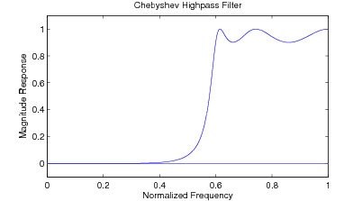
The specifications are given for a highpass Chebyshev frequency response with a passband edge at Hertz with a sampling rate of one sample per second. The order is set at and the passband ripple at 0.91515 dB. The transfer function is
The frequency response plot is given in [link] .
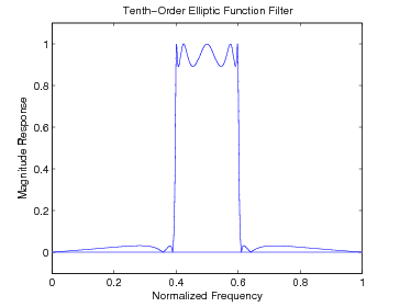
This filter requires a bandpass frequency response with an elliptic-function approximation. The maximum passpand ripple is one dB,the minimum stopband attenuation is 30 dB, the lower stopband edge , the lower passband edge , the upper passband edge , and the upper stopband edge Hertz with a sampling rate of one sample per second. The design program calculated a requiredprototype order of and, therefore, a total order of 10. The frequency response plot is shown in [link] .
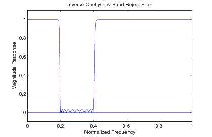
The specifications are given for a bandreject Inverse- Chebyshev frequency response with bandedges at and Hertz with a sampling rate of one sample per second. The order is set at and the minimum stopband attenuation at 30 dB. The frequency response plot is given in [link] .
This section has described the two most popular and useful methods for transforming a prototype analog filter into a digitalfilter. The analog frequency variable is used because a literature on analog filter design exists, but more importantly,many approximation theories are more straightforward in terms of the Laplace-transform variable than the z-transform variable. Theimpulse-invariant method is particularly valuable when time- domain characteristics are important. The bilinear-transformmethod is the most common when frequency-domain performance is the main interest. Use of the BLT warps the frequency scale and,therefore, the digital band edges must be prewarped to obtain the necessary band edges for the analog filter design. Formulas thattransform the analog prototype filters into the desired digital filters and for prewarping specifications were derived.
The use of frequency transformations to convert lowpass filters into highpass, bandpass, and bandreject filters wasdiscussed as a particularly useful combination with the bilinear transformation. These are implemented in Program 8 and designexamples from this program were shown.
There are cases where no analytic results are possible or where the desired frequency response is not piecewise constant andtransformation methods are not appropriate. Direct methods for these cases are developed in other sections.
Notification Switch
Would you like to follow the 'Digital signal processing and digital filter design (draft)' conversation and receive update notifications?

|
|

|
|

|
|

|
|

|
|

|
|

|
|

|
|

|
|

|