3.6 Frequency transformations

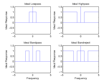
In addition to the lowpass frequency response, other basic ideal responses are often needed in practice. The ideal highpass filterrejects signals with frequencies below a certain value and passes those with frequencies above that value. The ideal bandpass filter passes only aband of frequencies, and the ideal band reject filter completely rejects a band of frequencies. These ideal frequency responses are illustrated in [link] .

This section presents a method for designing the three new filters by using a frequency transformation on the basic lowpass design. When used onthe four classical IIR approximations (e.g. Butterworth, Chebyshev, inverse-Chebyshev, and Elliptic Function), the optimality is preserved.This procedure is used in the FREQXFM() subroutine of Program 8 in the appendix.

Change the bandedge

The classical filters have all been developed for a bandedge of ${\omega }_0=1$ . That is where the Butterworth filter has a magnitude squared of one half: $\left|F\right|=0.5$ or the Chebyshev filter has its passband edge or the Inverse Chebyshev has its stopband edge or the Elliptic filterhas its passband edge. To scale the bandedge, simply replace $s$ by $Ks$ or: $s\to Ks$ where $K$ is reciprocal of the new desired bandedge. What happened to the prototype filter at $\omega =1$ will now happen at $\omega =1/K$ . It is simply a linear scaling of the $\omega$ axis. This change can be done before the conversions below or after.

The highpass filter

The frequency response illustrated in [link] b can be obtained from that in [link] a by replacing the complex frequency variable $s$ in the transfer function by $1/s$ . This change of variable maps zero frequency to infinity, maps unity into unity, andmaps infinity to zero. It turns the complex $s$ plane inside out and leaves the unit circle alone.

In the design procedure, the desired bandedge ${\omega }_0$ for the highpass filter is mapped by $1/{\omega }_0$ to give the bandedge for the prototype lowpass filter. This lowpass filter is next designed byone of the optimal procedures already covered and then converted to a highpass transfer function by replacing $s$ by $1/s$ . If an elliptic-function filter approximation is used, both the passbandedge ${\omega }_p$ and the stopbandedge ${\omega }_s$ are transformed. Because most optimal lowpass design procedures give the designed transferfunction in factored form from explicit formulas for the poles and zeros, the transformation can be performed on each pole andzero to give the highpass transfer function in factored form.

The bandpass filter

In order to convert the lowpass filter of [link] a into that of [link] c, a more complicated frequency transformation is required. In order to reduce confusion, the complexfrequency variable for the prototype analog filter transfer function will be denoted by $p$ and that for the transformed analog filter by $s$ . The transformation is given by

This change of variables doubles the order of the filter, maps the origin of the $s$ -plane to both plus and minus $j{\omega }_0$ , and maps minus and plus infinity to zero and infinity. The entire $\omega$ axis of the prototype response is mapped between zero and plus infinity on thetransformed responses. It is also mapped onto the left-half axis between minus infinity and zero. This is illustrated in [link] .