

| << Chapter < Page | Chapter >> Page > |
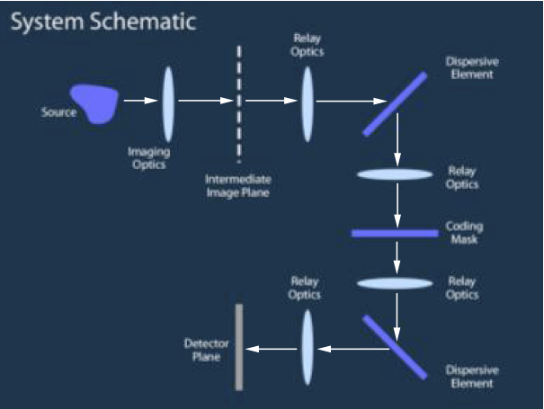
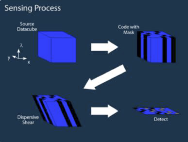
The dual disperser coded aperture snapshot spectral imager (DD-CASSI), shown in [link] , is an architecture that combines separate multiplexing in the spatial and spectral domain, which is then sensed by a wide-wavelength sensor/pixel array, thus flattening the spectral dimension [link] .
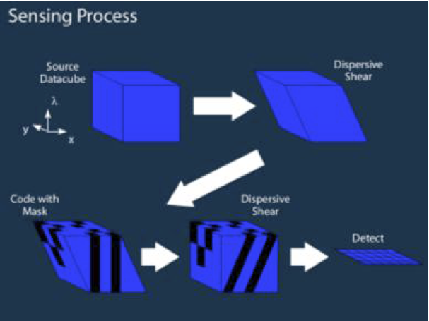
First, a dispersive element separates the different spectral bands, which still overlap in the spatial domain. In simple terms, this element shears the datacube, with each spectral slice being displaced from the previous by a constant amount in the same spatial dimension. The resulting datacube is then masked using the coded aperture, whose effect is to "punch holes" in the sheared datacube by blocking certain pixels of light. Subsequently, a second dispersive element acts on the masked, sheared datacube; however, this element shears in the opposite direction, effectively inverting the shearing of the first dispersive element. The resulting datacube is upright, but features "sheared" holes of datacube voxels that have been masked out.
The resulting modified datacube is then received by a sensor array, which flattens the spectral dimension by measuring the sum of all the wavelengths received; the received light field resembles the target image, allowing for optical adjustments such as focusing. In this way, the measurements consist of full sampling in the spatial and dimensions, with an aggregation effect in the spectral dimension.
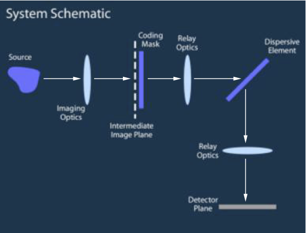
The single disperser coded aperture snapshot spectral imager (SD-CASSI), shown in [link] , is a simplification of the DD-CASSI architecture in which the first dispersive element is removed [link] . Thus, the light field received at the sensors does not resemble the target image. Furthermore, since the shearing is not reversed, the area occupied by the sheared datacube is larger than that of the original datacube, requiring a slightly larger number of pixels for the capture.
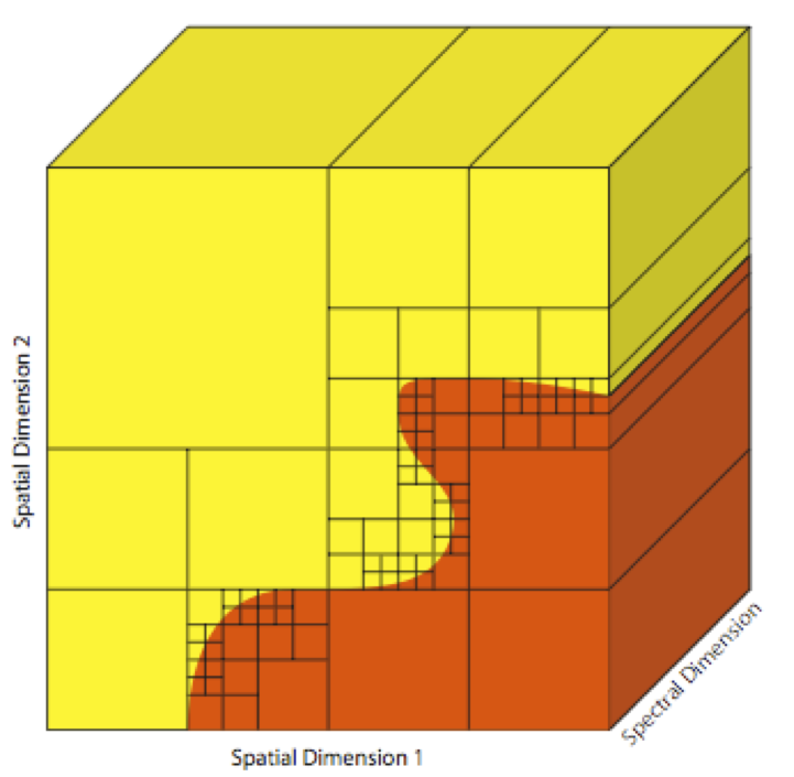
This sparsity structure assumes that the spectral signature for all pixels in a neighborhood is close to constant; that is, that the datacube is piecewise constant with smooth borders in the spatial dimensions. The complexity of an image is then given by the number of spatial dyadic squares with constant spectral signature necessary to accurately approximate the datacube; see [link] . A reconstruction algorithm then searches for the signal of lowest complexity (i.e., with the fewest dyadic squares) that generates compressive measurements close to those observed [link] .
This sparsity structure operates on each spectral band separately and assumes the same type of sparsity structure for each band [link] . The sparsity basis is drawn from those commonly used in images, such as wavelets, curvelets, or the discrete cosine basis. Since each basis operates only on a band, the resulting sparsity basis for the datacube can be represented as a block-diagonal matrix:
This sparsity structure employs separate sparsity bases for the spatial dimensions and the spectral dimension, and builds a sparsity basis for the datacube using the Kronecker product of these two [link] :
In this manner, the datacube sparsity bases simultaneously enforces both spatial and spectral structure, potentially achieving a sparsity level lower than the sums of the spatial sparsities for the separate spectral slices, depending on the level of structure between them and how well can this structure be captured through sparsity.
Compressive sensing will make the largest impact in applications with very large, high dimensional datasets that exhibit considerable amounts of structure. Hyperspectral imaging is a leading example of such applications; the sensor architectures and data structure models surveyed in this module show initial promising work in this new direction, enabling new ways of simultaneously sensing and compressing such data. For standard sensing architectures, the data structures surveyed also enable new transform coding-based compression schemes.
Notification Switch
Would you like to follow the 'An introduction to compressive sensing' conversation and receive update notifications?

|
|

|
|
|
|
|
|
|
|
|
|
|
|
|

|
|

|
|

|
|

|