2.2 Sparse representations

Transforming a signal to a new basis or frame may allow us to represent a signal more concisely. The resulting compression is useful for reducing data storage and data transmission, which can be quite expensive in some applications. Hence, one might wish to simply transmit the analysis coefficients obtained in our basis or frame expansion instead of its high-dimensional correlate. In cases where the number of non-zero coefficients is small, we say that we have a sparse representation. Sparse signal models allow us to achieve high rates of compression and in the case of compressive sensing , we may use the knowledge that our signal is sparse in a known basis or frame to recover our original signal from a small number of measurements. For sparse data, only the non-zero coefficients need to be stored or transmitted in many cases; the rest can be assumed to be zero).

Mathematically, we say that a signal $x$ is $K$ -sparse when it has at most $K$ nonzeros, i.e., ${∥x∥}_0\le K$ . We let

denote the set of all $K$ -sparse signals. Typically, we will be dealing with signals that are not themselves sparse, but which admit a sparse representation in some basis $\Psi$ . In this case we will still refer to $x$ as being $K$ -sparse, with the understanding that we can express $x$ as $x=\Psi \alpha$ where ${\parallel \alpha \parallel }_0\le K$ .

Sparsity has long been exploited in signal processing and approximation theory for tasks such as compression  [link] , [link] , [link] and denoising  [link] , and in statistics and learning theory as a method for avoiding overfitting  [link] . Sparsity also figures prominently in the theory of statistical estimation and model selection  [link] , [link] , in the study of the human visual system  [link] , and has been exploited heavily in image processing tasks, since the multiscale wavelet transform  [link] provides nearly sparse representations for natural images. Below, we briefly describe some one-dimensional (1-D) and two-dimensional (2-D) examples.

1-d signal models

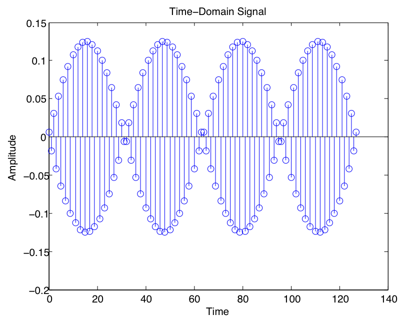
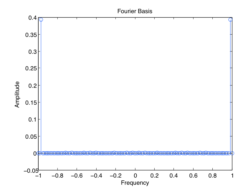
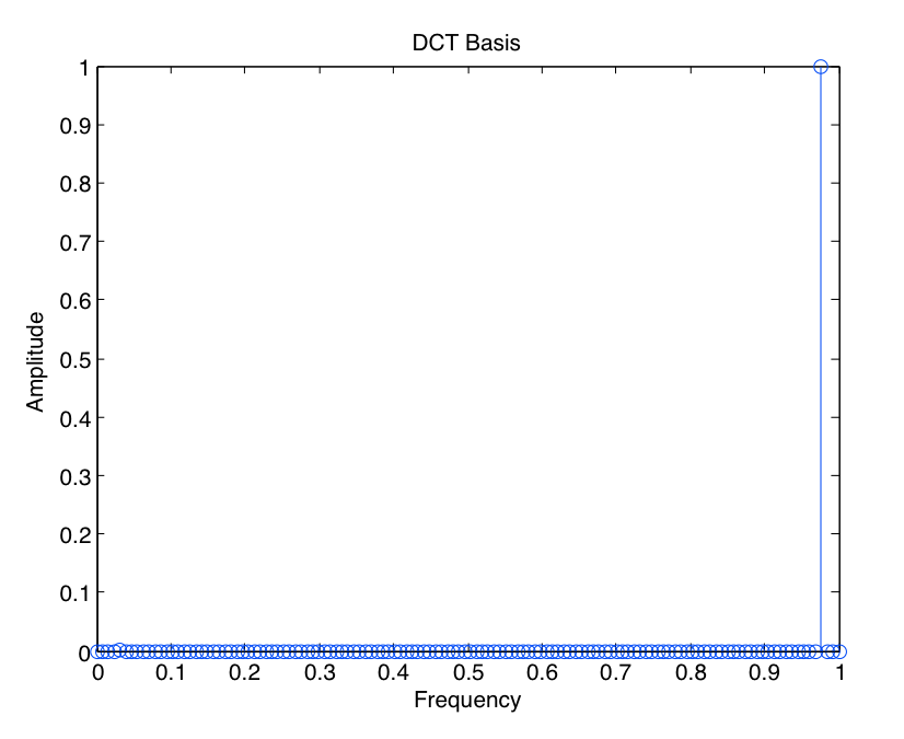
We will now present an example of three basis expansions that yield different levels of sparsity for the same signal. A simple periodic signal is sampled and represented as a periodic train of weighted impulses (see [link] ). One can interpret sampling as a basis expansion where our elements in our basis are impulses placed at periodic points along the time axis. We know that in this case, our dual basis consists of sinc functions used to reconstruct our signal from discrete-time samples. This representation contains many non-zero coefficients, and due to the signal's periodicity, there are many redundant measurements. Representing the signal in the Fourier basis, on the other hand, requires only two non-zero basis vectors, scaled appropriately at the positive and negative frequencies (see [link] ). Driving the number of coefficients needed even lower, we may apply the discrete cosine transform (DCT) to our signal, thereby requiring only a single non-zero coefficient in our expansion (see [link] ). The DCT equation is $X_k={\sum }_{n=0}^{N-1}{x}_{n}cos\left(\frac{\pi }{N}(n+\frac{1}{2})k\right)$ with $k=0,\cdots ,N-1$ , $x_n$ the input signal, and N the length of the transform.

2-d signal models

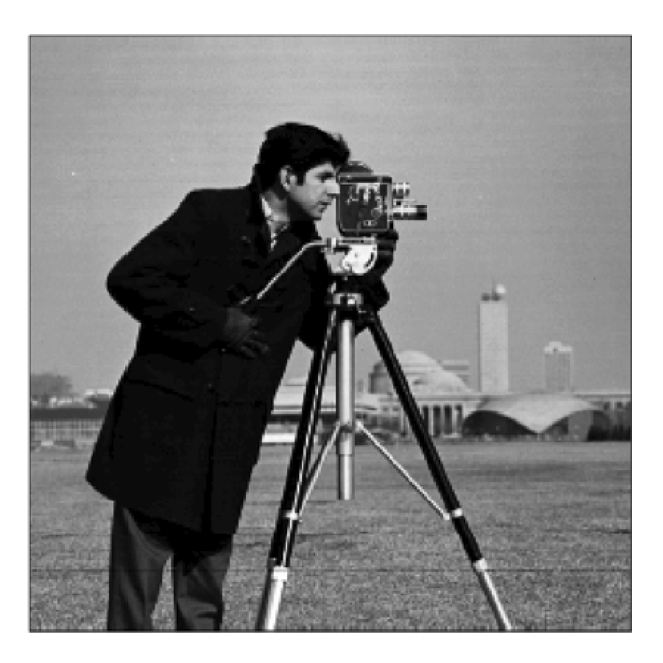
This same concept can be extended to 2-D signals as well. For instance, a binary picture of a nighttime sky is sparse in the standard pixel domain because most of the pixels are zero-valued black pixels. Likewise, natural images are characterized by large smooth or textured regions and relatively few sharp edges. Signals with this structure are known to be very nearly sparse when represented using a multiscale wavelet transform  [link] . The wavelet transform consists of recursively dividing the image into its low- and high-frequency components. The lowest frequency components provide a coarse scale approximation of the image, while the higher frequency components fill in the detail and resolve edges. What we see when we compute a wavelet transform of a typical natural image, as shown in [link] , is that most coefficients are very small. Hence, we can obtain a good approximation of the signal by setting the small coefficients to zero, or thresholding the coefficients, to obtain a $K$ -sparse representation. When measuring the approximation error using an ${\ell }_p$ norm, this procedure yields the best $K$ -term approximation of the original signal, i.e., the best approximation of the signal using only $K$ basis elements. Thresholding yields the best $K$ -term approximation of a signal with respect to an orthonormal basis. When redundant frames are used, we must rely on sparse approximation algorithms like those described later in this course  [link] , [link] .

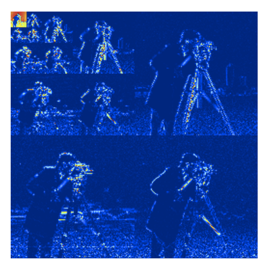
Sparsity results through this decomposition because in most natural images most pixel values vary little from their neighbors. Areas with little contrast difference can be represent with low frequency wavelets. Low frequency wavelets are created through stretching a mother wavelet and thus expanding it in space. On the other hand, discontinuities, or edges in the picture, require high frequency wavelets, which are created through compacting a mother wavelet. At the same time, the transitions are generally limited in space, mimicking the properties of the high frequency compacted wavelet. See "Compressible signals" for an example.