4.8 Lagrange multipliers

Solving optimization problems for functions of two or more variables can be similar to solving such problems in single-variable calculus. However, techniques for dealing with multiple variables allow us to solve more varied optimization problems for which we need to deal with additional conditions or constraints. In this section, we examine one of the more common and useful methods for solving optimization problems with constraints.

Lagrange multipliers

[link] was an applied situation involving maximizing a profit function, subject to certain constraints . In that example, the constraints involved a maximum number of golf balls that could be produced and sold in $1$ month $\left(x\right),$ and a maximum number of advertising hours that could be purchased per month $\left(y\right).$ Suppose these were combined into a budgetary constraint, such as $20x+4y\le 216,$ that took into account the cost of producing the golf balls and the number of advertising hours purchased per month. The goal is, still, be to maximize profit, but now there is a different type of constraint on the values of $x$ and $y.$ This constraint, when combined with the profit function $f\left(x,y\right)=48x+96y-x^2-2xy-9y^2,$ is an example of an optimization problem    , and the function $f\left(x,y\right)$ is called the objective function    . A graph of various level curves of the function $f\left(x,y\right)$ follows.

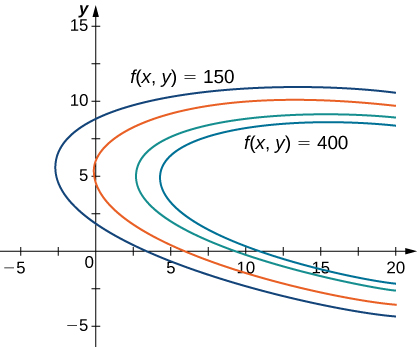
In [link] , the value $c$ represents different profit levels (i.e., values of the function $f).$ As the value of $c$ increases, the curve shifts to the right. Since our goal is to maximize profit, we want to choose a curve as far to the right as possible. If there was no restriction on the number of golf balls the company could produce, or the number of units of advertising available, then we could produce as many golf balls as we want, and advertise as much as we want, and there would be not be a maximum profit for the company. Unfortunately, we have a budgetary constraint that is modeled by the inequality $20x+4y\le 216.$ To see how this constraint interacts with the profit function, [link] shows the graph of the line $20x+4y=216$ superimposed on the previous graph.

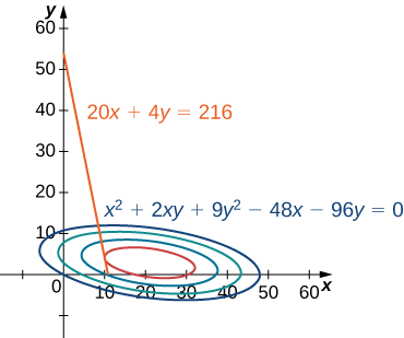
As mentioned previously, the maximum profit occurs when the level curve is as far to the right as possible. However, the level of production corresponding to this maximum profit must also satisfy the budgetary constraint, so the point at which this profit occurs must also lie on (or to the left of) the red line in [link] . Inspection of this graph reveals that this point exists where the line is tangent to the level curve of $f.$ Trial and error reveals that this profit level seems to be around $395,$ when $x$ and $y$ are both just less than $5.$ We return to the solution of this problem later in this section. From a theoretical standpoint, at the point where the profit curve is tangent to the constraint line, the gradient of both of the functions evaluated at that point must point in the same (or opposite) direction. Recall that the gradient of a function of more than one variable is a vector. If two vectors point in the same (or opposite) directions, then one must be a constant multiple of the other. This idea is the basis of the method of Lagrange multipliers    .