4.1 Basics of differential equations (Page 3/14)

Calculus volume 2 Page 3 / 14

A differential equation together with one or more initial values is called an initial-value problem . The general rule is that the number of initial values needed for an initial-value problem is equal to the order of the differential equation. For example, if we have the differential equation $y^{'} = 2 x,$ then $y (3) = 7$ is an initial value, and when taken together, these equations form an initial-value problem. The differential equation $y ″ - 3 y^{'} + 2 y = 4 e^{x}$ is second order, so we need two initial values. With initial-value problems of order greater than one, the same value should be used for the independent variable. An example of initial values for this second-order equation would be $y (0) = 2$ and $y^{'} (0) = −1 .$ These two initial values together with the differential equation form an initial-value problem. These problems are so named because often the independent variable in the unknown function is $t,$ which represents time. Thus, a value of $t = 0$ represents the beginning of the problem.

Verifying a solution to an initial-value problem

Verify that the function $y = 2 e^{−2 t} + e^{t}$ is a solution to the initial-value problem

y^{'} + 2 y = 3 e^{t}, y (0) = 3 .

For a function to satisfy an initial-value problem, it must satisfy both the differential equation and the initial condition. To show that $y$ satisfies the differential equation, we start by calculating $y^{'} .$ This gives $y^{'} = −4 e^{−2 t} + e^{t} .$ Next we substitute both $y$ and $y^{'}$ into the left-hand side of the differential equation and simplify:

\begin{matrix} y^{'} + 2 y & = (−4 e^{−2 t} + e^{t}) + 2 (2 e^{−2 t} + e^{t}) \\ = −4 e^{−2 t} + e^{t} + 4 e^{−2 t} + 2 e^{t} \\ = 3 e^{t} . \end{matrix}

This is equal to the right-hand side of the differential equation, so $y = 2 e^{−2 t} + e^{t}$ solves the differential equation. Next we calculate $y (0) :$

\begin{matrix} y (0) & = 2 e^{−2 (0)} + e^{0} \\ = 2 + 1 \\ = 3 . \end{matrix}

This result verifies the initial value. Therefore the given function satisfies the initial-value problem.

Got questions? Get instant answers now!

Verify that $y = 3 e^{2 t} + 4 sin t$ is a solution to the initial-value problem

y^{'} - 2 y = 4 cos t - 8 sin t, y (0) = 3 .

Got questions? Get instant answers now!

In [link] , the initial-value problem consisted of two parts. The first part was the differential equation $y^{'} + 2 y = 3 e^{x},$ and the second part was the initial value $y (0) = 3 .$ These two equations together formed the initial-value problem.

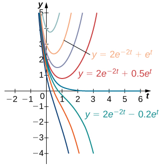
The same is true in general. An initial-value problem will consists of two parts: the differential equation and the initial condition. The differential equation has a family of solutions, and the initial condition determines the value of $C .$ The family of solutions to the differential equation in [link] is given by $y = 2 e^{−2 t} + C e^{t} .$ This family of solutions is shown in [link] , with the particular solution $y = 2 e^{−2 t} + e^{t}$ labeled.

A graph of a family of solutions to the differential equation y’ + 2 y = 3 e ^ t, which are of the form y = 2 e ^ (-2 t) + C e ^ t. The versions with C = 1, 0.5, and -0.2 are shown, among others not labeled. For all values of C, the function increases rapidly for t < 0 as t goes to negative infinity. For C > 0, the function changes direction and increases in a gentle curve as t goes to infinity. Larger values of C have a tighter curve closer to the y axis and at a higher y value. For C = 0, the function goes to 0 as t goes to infinity. For C < 0, the function continues to decrease as t goes to infinity. — A family of solutions to the differential equation $y^{'} + 2 y = 3 e^{t} .$ The particular solution $y = 2 e^{−2 t} + e^{t}$ is labeled.

Solving an initial-value problem

Solve the following initial-value problem:

y^{'} = 3 e^{x} + x^{2} - 4, y (0) = 5 .

The first step in solving this initial-value problem is to find a general family of solutions. To do this, we find an antiderivative of both sides of the differential equation

\int y^{'} d x = \int (3 e^{x} + x^{2} - 4) d x,

namely,

y + C_{1} = 3 e^{x} + \frac{1}{3} x^{3} - 4 x + C_{2} .

We are able to integrate both sides because the y term appears by itself. Notice that there are two integration constants: $C_{1}$ and $C_{2} .$ Solving [link] for $y$ gives

y = 3 e^{x} + \frac{1}{3} x^{3} - 4 x + C_{2} - C_{1} .

Because $C_{1}$ and $C_{2}$ are both constants, $C_{2} - C_{1}$ is also a constant. We can therefore define $C = C_{2} - C_{1},$ which leads to the equation

y = 3 e^{x} + \frac{1}{3} x^{3} - 4 x + C .

Next we determine the value of $C .$ To do this, we substitute $x = 0$ and $y = 5$ into [link] and solve for $C :$

\begin{matrix} 5 & = & 3 e^{0} + \frac{1}{3} 0^{3} - 4 (0) + C \\ 5 & = & 3 + C \\ C & = & 2 . \end{matrix}

Now we substitute the value $C = 2$ into [link] . The solution to the initial-value problem is $y = 3 e^{x} + \frac{1}{3} x^{3} - 4 x + 2 .$

Got questions? Get instant answers now!

<< Chapter < Page Page > Chapter >>

Practice Key Terms 8

Read also:

Get Jobilize Job Search Mobile App in your pocket Now!

100% Free Mobile Applications
Receive real-time job alerts and never miss the right job again

Source: OpenStax, Calculus volume 2. OpenStax CNX. Feb 05, 2016 Download for free at http://cnx.org/content/col11965/1.2

Google Play and the Google Play logo are trademarks of Google Inc.

Notification Switch

Would you like to follow the 'Calculus volume 2' conversation and receive update notifications?

Ask

	10 Biology 10 Cell Reproduction MCQ By OpenStax Start Quiz
	Does your crush like you? By Hoy Wen Start Quiz
	3 Neuroscience Exam 2004 4 By David Corey Start Exam
©flickr: Bertram	Chemistry Ch 1 2 Test 1 By Madison Christian Start Quiz
©flickr: quinn	Neuroanatomy By George Turner Start Quiz
	3 Microbiology Final 3 By Madison Christian Start Test
	Excel 2007 Quiz By Lakeima Roberts Start Quiz
	13 AP Key Terms 13 Anatomy of the Nervous System By OpenStax Start Key Terms
	Job Search Skills MCQ By Mary Matera Start Quiz
	17 AP Key Terms 17 Endocrine System By OpenStax Start Key Terms