2.2 Least squared error design of fir filters  (Page 12/13)

Matlab programs

A Matlab program for designing multiband FIR filters using the weighted least squares approximation described in [link] and [link] above is included in the Appendix. The program assumes passbands and stopbandsthat alternate with transition bands. The passbands are assumed to have constant gain for simplicity but that could be generalized with theresults from FIR Digital Filters . The first for loop constructs the ${\widehat{h}}_w\left(n\right)$ in [link] by sequentially designing weighted bandpass filters and a separately weighted transition band similar to the examplein [link] . These are added together in this loop to give the vector $h_w$ in [link] . The second for loop constructs the $\mathbf{C}$ matrix in [link] using the formula [link] . Care must be taken to correctly calculate the indeterminate values of sinc(0) and to properlyinclude the effects of ${\omega }_F=\pi$ .

When one uses zero weights in the transition bands, the $\mathbf{C}$ matrix becomes ill conditioned when the product of the filter length $N$ and the sum of the transition band widths in Hertz is much above 12. This is anapproximate rule which is somewhat affected by different passband and stopband weights, but it gives an indication of when numerical problemswill occur. To reduce this problem, the program includes optimal spline transition functions so that a small weight can be used to improve theconditioning of $\mathbf{C}$ with minimal effect on the optimality of the approximation.

Examples

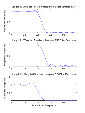
To illustrate the effects of using a weighted least squared error design criterion, a simple length-21 linear phase lowpass FIR filter wasdesigned, with unity weighting in the pass and stop bands and zero weighting in the transition band. The frequency response is shown in [link] a. The same filter is designed with a weight of 100 in the passband and the response is shown in [link] b and the case for a weight of 100 in the stopband is shown in [link] c. It is instructive to design many example filters and observe the effectsof different weights, use of spline vs zero weight transition bands, and the effects of the transition band width on the pass and stopbandperformance.

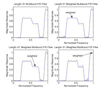
The same specifications that were used in the design using optimal spline transition functions of [link] a is used in the design here with unity weights in the stop and passbands and zero weights in thetransition bands. The result is fairly similar to the spline function design and is shown in [link] a for $N=51$ . For lengths above around 131, numerical errors resulted in erratic performance in thetransition bands. Indeed for this case, the use of the spline method would probably be superior. The advantage of the weighted least squares methodis illustrated in [link] b where the same specifications are used but with a weight of 100 in the first passband, in [link] c where a weight of 100 is used in the second passband, and in [link] d where a weight of 100 is used in the third passband. This use of weights is impossible using the spline method or anywindowing method.