

| << Chapter < Page | Chapter >> Page > |
An example of the use of a dummy variable is the work estimating the impact of gender on salaries. There is a full body of literature on this topic and dummy variables are used extensively. For this example the salaries of elementary and secondary school teachers for a particular state is examined. Using a homogeneous job category, school teachers, and for a single state reduces many of the variations that naturally effect salaries such as differential physical risk and other working conditions. The estimating equation in its simplest form specifies salary as a function of various teacher characteristic that economic theory would suggest could affect salary. These would include education level as a measure of potential productivity, age and/or experience to capture on-the-job training, again as a measure of productivity. Because the data are for school teachers employed in a public school districts rather than workers in a for-profit company, the school district’s average revenue per average daily student attendance is included as a measure of ability to pay. The results of the regression analysis using data on 24,916 school teachers are presented below.
| Variable | Regression Coefficients (b) | Standard Errors of the Estimates
for Teacher's Earnings Function (s b ) |
|---|---|---|
| Intercept | 4269.9 | |
| Gender (male = 1) | 632.38 | 13.39 |
| Total Years of Experience | 52.32 | 1.10 |
| Years of Experience in Current District | 29.97 | 1.52 |
| Education | 629.33 | 13.16 |
| Total Revenue per ADA | 90.24 | 3.76 |
| .725 | ||
| n | 24,916 |
The coefficients for all the independent variables are significantly different from zero as indicated by the standard errors. Dividing the standard errors of each coefficient results in a t-value greater than 1.96 which is the required level for 95% confidence. The binary variable, our dummy variable of interest in this analysis, is gender where male is given a value of 1 and female given a value of 0. The coefficient is significantly different from zero with a dramatic t-statistic of 47 standard deviations. We thus cannot accept the null hypothesis that the coefficient is equal to zero. Therefore we conclude that there is a premium paid male teachers of $632 after holding constant experience, education and the wealth of the school district in which the teacher is employed. It is important to note that these data are from some time ago and the $632 represents a six percent salary premium. A graph of this example of dummy variables is presented below.
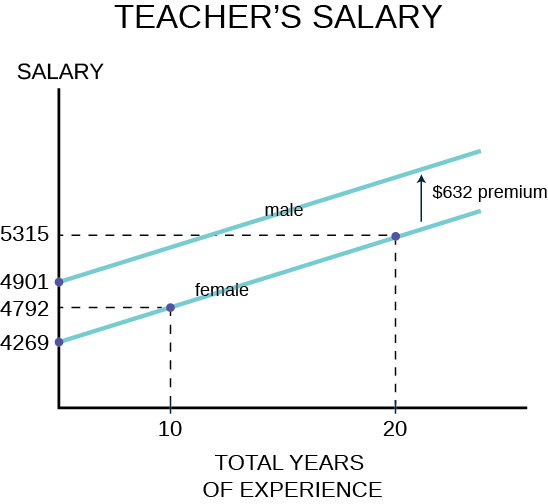
In two dimensions, salary is the dependent variable on the vertical axis and total years of experience was chosen for the continuous independent variable on horizontal axis. Any of the other independent variables could have been chosen to illustrate the effect of the dummy variable. The relationship between total years of experience has a slope of $52.32 per year of experience and the estimated line has an intercept of $4,269 if the gender variable is equal to zero, for female. If the gender variable is equal to 1, for male, the coefficient for the gender variable is added to the intercept and thus the relationship between total years of experience and salary is shifted upward parallel as indicated on the graph. Also marked on the graph are various points for reference. A female school teacher with 10 years of experience receives a salary of $4,792 on the basis of her experience only, but this is still $109 less than a male teacher with zero years of experience.
Notification Switch
Would you like to follow the 'Introductory statistics' conversation and receive update notifications?

|
|
|
|
|

|
|

|
|

|
|

|
|

|
|

|
|

|
|

|