0.4 Limits to growth

A limit to simple growth: the logistic function

In the preceding sections we saw how the linear first-order differential equations lead to exponential solutions. Both the unbounded nature of thesolution and the assumption of a constant growth rate indicate a modification that will give more realistic modeling of observed populationgrowths.

• A A Nonlinear Equation

It seems reasonable to assume under that many conditions the growth rate $r$ would not remain constant, but would decrease with increasing population.This might result from the effects of crowding and reduced resources, or other physical and psychological factors on the birth and death rates.The simpliest functional form one could assume would be a linear reduction of $r$ as the population increased.

Here $r_o$ is the rate for very small $p$ where no limits have been felt.The term $\beta$ gives the reducing effect of $p$ on $r$ . This is seen by plotting $r$ versus $p$ .

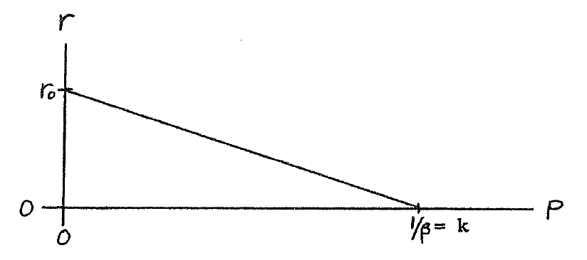
This is now a nonlinear first-order differential equation with several interesting features.The solution of [link] can be shown to equal

for

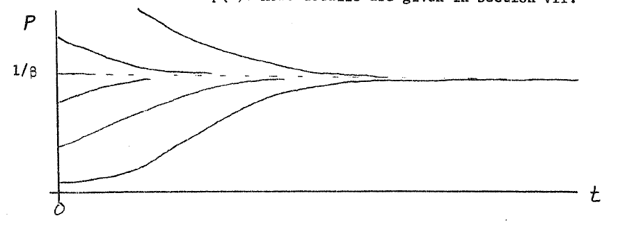
This function is called a logistic or sigmoid, and is illustrated below for several initial values of $p\left(o\right)$ .

An alternate form is

where $k$ is $p\left(\infty \right)$ , the asymptotic value of population, or the carrying capacity of the "system".This requires $k=\frac{1}{\beta }$ .

There are several very interesting features of this function. For small initial populations, the initial increase is very much likeexponential. This is obvious since the negative term in [link] is small and the equation looks linear.However, as $p\left(t\right)$ grows, the growth rate goes to zero and a steady-state or equilibrium is approached as a limit.

It it interesting to note that it is possible to normalize the logistic into a "standard" form.If we scale both the amplitude and time by

then [link] becomes

When plotted on semi-log paper, the logistic is an increasing straightline for small time, and becomes a horizontal straight line for large time.

The use of the logistic to model simple population growth with a limit is shown in Figures 4, 5, and 6.There have been many other applications of the logistic [link] [link] [link] [link] with some success and some failures. Unfortunately, if one tries to use this model to predict the limitingvalue while the system is still in the early stages of growth, a large error results since an exponential and a logistic look very similar inthe early stages.

It is possible to manipulate the data so that a plot of it becomes a straight line.If the reciprocal of $p\left(t\right)$ in [link] is considered

and the logarithm is taken

we have a linear function. Unfortunately, trial-and-error must be used to find $\beta$ since it appears on both sides of the [link] .

A more complicated limit to growth

The [link] that gives rise to the logistic is the simpliest modification to include the effect of a non-constant $r$ . Perhaps a more realistic relation of $r$ as a function of $p$ could be found.In general, the equation becomes

where $f\left(p\right)$ is a more complicated function of $p$ . The nature of the solution will still be the same in the sensethat $p\left(t\right)$ will move from an initial value monotonically toward a constant limit – there can be no over or under shoots with the model.There may be more than one possible final steady-state value if $f\left(p\right)$ has more than one zero.

Consider the growth rate to vary as a quadratic function of population rather than as a linear function shown in [link] . One particular form it might take could be

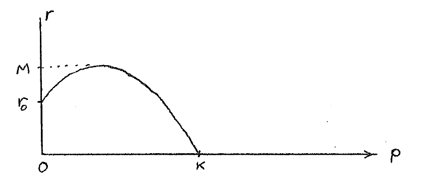
where

This might be the model of a system where moderate increases in population increase the growth rate, but higher values finally causethe rate to drop as before. A situation where moderate levels allow male and female members to find each other more often could lead to this model, or a process such asindustrialization, where efficiency can increase with size to a point.

The resulting differential equation is first order, but now has a cubic nonlinearity.

The solution looks somewhat like a logistic. It starts with low population and an exponential growth;then, as the second term begins to dominate, the growth is super-exponential – faster than exponential.Finally, the cubic term – the limit – causes an abrupt leveling off to a constant equilibrium value of $k$ .

If more complicated systems are to be modeled, modification other than more complicated nonlinearities must be used.Other modification might include

• a Time delays
• b Use population age groups
• c Allow parameters to depend on other environmental variables or states.

The next generalization we will consider here will be the addition of another state variable.This allows a much broader and more versatile system of equations and solutions.