<< Chapter < Page Chapter >> Page >

Evaluate the integral R x e x y d A where R = [ 0 , 1 ] × [ 0 , ln 5 ] .

4 ln 5 ln 5

Got questions? Get instant answers now!

Applications of double integrals

Double integrals are very useful for finding the area of a region bounded by curves of functions. We describe this situation in more detail in the next section. However, if the region is a rectangular shape, we can find its area by integrating the constant function f ( x , y ) = 1 over the region R .

Definition

The area of the region R is given by A ( R ) = R 1 d A .

This definition makes sense because using f ( x , y ) = 1 and evaluating the integral make it a product of length and width. Let’s check this formula with an example and see how this works.

Finding area using a double integral

Find the area of the region R = { ( x , y ) | 0 x 3 , 0 y 2 } by using a double integral, that is, by integrating 1 over the region R .

The region is rectangular with length 3 and width 2, so we know that the area is 6. We get the same answer when we use a double integral:

A ( R ) = 0 2 0 3 1 d x d y = 0 2 [ x | 0 3 ] d y = 0 2 3 d y = 3 0 2 d y = 3 y | 0 2 = 3 ( 2 ) = 6 .
Got questions? Get instant answers now!

We have already seen how double integrals can be used to find the volume of a solid bounded above by a function f ( x , y ) over a region R provided f ( x , y ) 0 for all ( x , y ) in R . Here is another example to illustrate this concept.

Volume of an elliptic paraboloid

Find the volume V of the solid S that is bounded by the elliptic paraboloid 2 x 2 + y 2 + z = 27 , the planes x = 3 and y = 3 , and the three coordinate planes.

First notice the graph of the surface z = 27 2 x 2 y 2 in [link] (a) and above the square region R 1 = [ −3 , 3 ] × [ −3 , 3 ] . However, we need the volume of the solid bounded by the elliptic paraboloid 2 x 2 + y 2 + z = 27 , the planes x = 3 and y = 3 , and the three coordinate planes.

This figure consists of two figures marked a and b. In figure a, in xyz space, the surface z = 20 minus 2x2 minus y2 is shown for x and y from negative 3 to positive 3. The shape looks like a sheet that has been pinned at the corners and forced up gently in the middle. In figure b, in xyz space, the surface z = 20 minus 2x2 minus y2 is shown for x and y from 0 to positive 3. The surface is the upper corner of the figure from part a, and below the surface is marked the solid S.
(a) The surface z = 27 2 x 2 y 2 above the square region R 1 = [ −3 , 3 ] × [ −3 , 3 ] . (b) The solid S lies under the surface z = 27 2 x 2 y 2 above the square region R 2 = [ 0 , 3 ] × [ 0 , 3 ] .

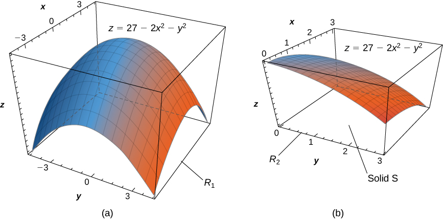
Now let’s look at the graph of the surface in [link] (b). We determine the volume V by evaluating the double integral over R 2 :

V = R z d A = R ( 27 2 x 2 y 2 ) d A = y = 0 y = 3 x = 0 x = 3 ( 27 2 x 2 y 2 ) d x d y Convert to iterated integral. = y = 0 y = 3 [ 27 x 2 3 x 3 y 2 x ] | x = 0 x = 3 d y Integrate with respect to x . = y = 0 y = 3 ( 64 3 y 2 ) d y = 63 y y 3 | y = 0 y = 3 = 162 .
Got questions? Get instant answers now!

Find the volume of the solid bounded above by the graph of f ( x , y ) = x y sin ( x 2 y ) and below by the x y -plane on the rectangular region R = [ 0 , 1 ] × [ 0 , π ] .

π 2

Got questions? Get instant answers now!

Recall that we defined the average value of a function of one variable on an interval [ a , b ] as

f ave = 1 b a a b f ( x ) d x .

Similarly, we can define the average value of a function of two variables over a region R . The main difference is that we divide by an area instead of the width of an interval.

Definition

The average value of a function of two variables over a region R is

f ave = 1 Area R R f ( x , y ) d x d y .

In the next example we find the average value of a function over a rectangular region. This is a good example of obtaining useful information for an integration by making individual measurements over a grid, instead of trying to find an algebraic expression for a function.

Calculating average storm rainfall

The weather map in [link] shows an unusually moist storm system associated with the remnants of Hurricane Karl, which dumped 4–8 inches (100–200 mm) of rain in some parts of the Midwest on September 22–23, 2010. The area of rainfall measured 300 miles east to west and 250 miles north to south. Estimate the average rainfall over the entire area in those two days.

A map of Wisconsin and Minnesota that shows many cities with numbers affixed to them. The highest numbers come in a narrow band, and the map is colored accordingly. The map effectively looks like a contour map, but instead of elevations, it uses these numbers.
Effects of Hurricane Karl, which dumped 4–8 inches (100–200 mm) of rain in some parts of southwest Wisconsin, southern Minnesota, and southeast South Dakota over a span of 300 miles east to west and 250 miles north to south.

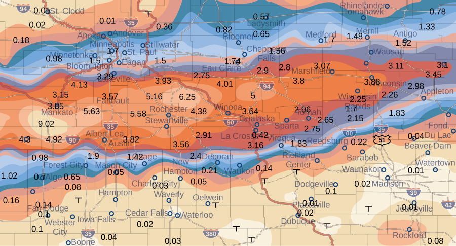
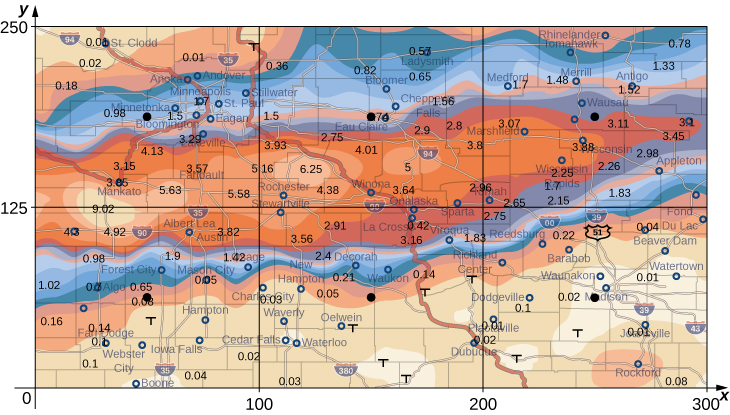
Place the origin at the southwest corner of the map so that all the values can be considered as being in the first quadrant and hence all are positive. Now divide the entire map into six rectangles ( m = 2 and n = 3 ) , as shown in [link] . Assume f ( x , y ) denotes the storm rainfall in inches at a point approximately x miles to the east of the origin and y miles to the north of the origin. Let R represent the entire area of 250 × 300 = 75000 square miles. Then the area of each subrectangle is

Δ A = 1 6 ( 75000 ) = 12500 .

Assume ( x i j * , y i j * ) are approximately the midpoints of each subrectangle R i j . Note the color-coded region at each of these points, and estimate the rainfall. The rainfall at each of these points can be estimated as:

At ( x 11 , y 11 ) the rainfall is 0.08.

At ( x 12 , y 12 ) the rainfall is 0.08.

At ( x 13 , y 13 ) the rainfall is 0.01.

At ( x 21 , y 21 ) the rainfall is 1.70.

At ( x 22 , y 22 ) the rainfall is 1.74.

At ( x 23 , y 23 ) the rainfall is 3.00.

Another version of the previous storm map, but this time with lines drawn for x = 100, 200, and 300 and for y = 125 and 250. There is a dot in the center of each of the resulting rectangles.
Storm rainfall with rectangular axes and showing the midpoints of each subrectangle.

According to our definition, the average storm rainfall in the entire area during those two days was

f ave = 1 Area R R f ( x , y ) d x d y = 1 75000 R f ( x , y ) d x d y 1 75,000 i = 1 3 j = 1 2 f ( x i j * , y i j * ) Δ A 1 75,000 [ f ( x 11 * , y 11 * ) Δ A + f ( x 12 * , y 12 * ) Δ A + f ( x 13 * , y 13 * ) Δ A + f ( x 21 * , y 21 * ) Δ A + f ( x 22 * , y 22 * ) Δ A + f ( x 23 * , y 23 * ) Δ A ] 1 75,000 [ 0.08 + 0.08 + 0.01 + 1.70 + 1.74 + 3.00 ] Δ A 1 75,000 [ 0.08 + 0.08 + 0.01 + 1.70 + 1.74 + 3.00 ] 12500 5 30 [ 0.08 + 0.08 + 0.01 + 1.70 + 1.74 + 3.00 ] 1.10.

During September 22–23, 2010 this area had an average storm rainfall of approximately 1.10 inches.

Got questions? Get instant answers now!
Practice Key Terms 4

Get Jobilize Job Search Mobile App in your pocket Now!

Get it on Google Play Download on the App Store Now


Source:  OpenStax, Calculus volume 3. OpenStax CNX. Feb 05, 2016 Download for free at http://legacy.cnx.org/content/col11966/1.2
Google Play and the Google Play logo are trademarks of Google Inc.

Notification Switch

Would you like to follow the 'Calculus volume 3' conversation and receive update notifications?

Ask