4.5 Derivatives and the shape of a graph  (Page 3/14)

Using the first derivative test

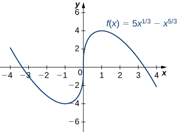
Use the first derivative test to find the location of all local extrema for $f\left(x\right)=5x^{1\text{/}3}-x^{5\text{/}3}.$ Use a graphing utility to confirm your results.

Step 1. The derivative is

$f^{\prime }\left(x\right)=\frac{5}{3}{x}^{\mathrm{-2}\text{/}3}-\frac{5}{3}{x}^{2\text{/}3}=\frac{5}{3x^{2\text{/}3}}-\frac{5x^{2\text{/}3}}{3}=\frac{5-5x^{4\text{/}3}}{3x^{2\text{/}3}}=\frac{5\left(1-x^{4\text{/}3}\right)}{3x^{2\text{/}3}}.$

The derivative $f^{\prime }\left(x\right)=0$ when $1-x^{4\text{/}3}=0.$ Therefore, $f^{\prime }\left(x\right)=0$ at $x=\text{±}1.$ The derivative $f^{\prime }\left(x\right)$ is undefined at $x=0.$ Therefore, we have three critical points: $x=0,$ $x=1,$ and $x=\mathrm{-1}.$ Consequently, divide the interval $\left(\text{−}\infty ,\infty \right)$ into the smaller intervals $\left(\text{−}\infty ,\mathrm{-1}\right),\left(\mathrm{-1},0\right),\left(0,1\right),$ and $\left(1,\infty \right).$

Step 2: Since $f^{\prime }$ is continuous over each subinterval, it suffices to choose a test point $x$ in each of the intervals from step $1$ and determine the sign of $f^{\prime }$ at each of these points. The points $x=\mathrm{-2},x=-\frac{1}{2},x=\frac{1}{2},\text{and}x=2$ are test points for these intervals.

Interval	Test Point	Sign of $f^{\prime }\left(x\right)=\frac{5\left(1-x^{4\text{/}3}\right)}{3x^{2\text{/}3}}$ at Test Point	Conclusion
$\left(\text{−}\infty ,\mathrm{-1}\right)$	$x=\mathrm{-2}$	$\frac{\left(\text{+}\right)\left(\text{−}\right)}{+}=\text{−}$	$f$ is decreasing.
$\left(\mathrm{-1},0\right)$	$x=-\frac{1}{2}$	$\frac{\left(\text{+}\right)\left(\text{+}\right)}{+}=+$	$f$ is increasing.
$\left(0,1\right)$	$x=\frac{1}{2}$	$\frac{\left(\text{+}\right)\left(\text{+}\right)}{+}=+$	$f$ is increasing.
$\left(1,\infty \right)$	$x=2$	$\frac{\left(\text{+}\right)\left(\text{−}\right)}{+}=\text{−}$	$f$ is decreasing.

Step 3: Since $f$ is decreasing over the interval $\left(\text{−}\infty ,\mathrm{-1}\right)$ and increasing over the interval $\left(\mathrm{-1},0\right),$ $f$ has a local minimum at $x=\mathrm{-1}.$ Since $f$ is increasing over the interval $\left(\mathrm{-1},0\right)$ and the interval $\left(0,1\right),$ $f$ does not have a local extremum at $x=0.$ Since $f$ is increasing over the interval $\left(0,1\right)$ and decreasing over the interval $\left(1,\infty \right),f$ has a local maximum at $x=1.$ The analytical results agree with the following graph.

Got questions? Get instant answers now!

Got questions? Get instant answers now!

Concavity and points of inflection

We now know how to determine where a function is increasing or decreasing. However, there is another issue to consider regarding the shape of the graph of a function. If the graph curves, does it curve upward or curve downward? This notion is called the concavity    of the function.

[link] (a) shows a function $f$ with a graph that curves upward. As $x$ increases, the slope of the tangent line increases. Thus, since the derivative increases as $x$ increases, $f^{\prime }$ is an increasing function. We say this function $f$ is concave up. [link] (b) shows a function $f$ that curves downward. As $x$ increases, the slope of the tangent line decreases. Since the derivative decreases as $x$ increases, $f^{\prime }$ is a decreasing function. We say this function $f$ is concave down.

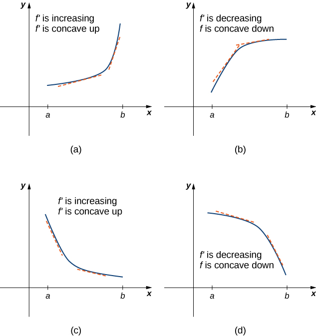
In general, without having the graph of a function $f,$ how can we determine its concavity? By definition, a function $f$ is concave up if $f^{\prime }$ is increasing. From Corollary $3,$ we know that if $f^{\prime }$ is a differentiable function, then $f^{\prime }$ is increasing if its derivative $f\text{″}\left(x\right)>0.$ Therefore, a function $f$ that is twice differentiable is concave up when $f\text{″}\left(x\right)>0.$ Similarly, a function $f$ is concave down if $f^{\prime }$ is decreasing. We know that a differentiable function $f^{\prime }$ is decreasing if its derivative $f\text{″}\left(x\right)<0.$ Therefore, a twice-differentiable function $f$ is concave down when $f\text{″}\left(x\right)<0.$ Applying this logic is known as the concavity test    .