18.3 Diameters of stars  (Page 3/4)

Diameters of eclipsing binary stars

We now turn back to the main thread of our story to discuss how all this can be used to measure the sizes of stars. The technique involves making a light curve of an eclipsing binary, a graph that plots how the brightness changes with time. Let us consider a hypothetical binary system in which the stars are very different in size, like those illustrated in [link] . To make life easy, we will assume that the orbit is viewed exactly edge-on.

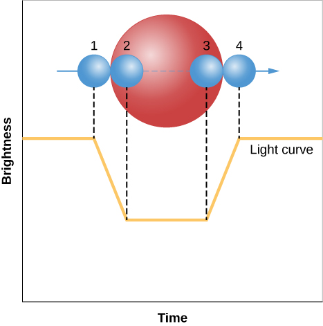
Even though we cannot see the two stars separately in such a system, the light curve can tell us what is happening. When the smaller star just starts to pass behind the larger star (a point we call first contact ), the brightness begins to drop. The eclipse becomes total (the smaller star is completely hidden) at the point called second contact . At the end of the total eclipse ( third contact ) , the smaller star begins to emerge. When the smaller star has reached last contact , the eclipse is completely over.

To see how this allows us to measure diameters, look carefully at [link] . During the time interval between the first and second contacts, the smaller star has moved a distance equal to its own diameter. During the time interval from the first to third contacts, the smaller star has moved a distance equal to the diameter of the larger star. If the spectral lines of both stars are visible in the spectrum of the binary, then the speed of the smaller star with respect to the larger one can be measured from the Doppler shift. But knowing the speed with which the smaller star is moving and how long it took to cover some distance can tell the span of that distance—in this case, the diameters of the stars. The speed multiplied by the time interval from the first to second contact gives the diameter of the smaller star. We multiply the speed by the time between the first and third contacts to get the diameter of the larger star.

Light curve of an edge-on eclipsing binary.

In actuality, the situation with eclipsing binaries is often a bit more complicated: orbits are generally not seen exactly edge-on, and the light from each star may be only partially blocked by the other. Furthermore, binary star orbits, just like the orbits of the planets, are ellipses, not circles. However, all these effects can be sorted out from very careful measurements of the light curve.

Using the radiation law to get the diameter

Another method for measuring star diameters makes use of the Stefan-Boltzmann law for the relationship between energy radiated and temperature (see Radiation and Spectra ). In this method, the energy flux (energy emitted per second per square meter by a blackbody, like the Sun) is given by

where σ is a constant and T is the temperature. The surface area of a sphere (like a star) is given by

The luminosity ( L ) of a star is then given by its surface area in square meters times the energy flux:

Previously, we determined the masses of the two stars in the Sirius binary system. Sirius gives off 8200 times more energy than its fainter companion star, although both stars have nearly identical temperatures. The extremely large difference in luminosity is due to the difference in radius, since the temperatures and hence the energy fluxes for the two stars are nearly the same. To determine the relative sizes of the two stars, we take the ratio of the corresponding luminosities:

Therefore, the relative sizes of the two stars can be found by taking the square root of the relative luminosity. Since $\sqrt{8200}=91$ , the radius of Sirius is 91 times larger than the radium of its faint companion.

The method for determining the radius shown here requires both stars be visible, which is not always the case.

Stellar diameters

The results of many stellar size measurements over the years have shown that most nearby stars are roughly the size of the Sun, with typical diameters of a million kilometers or so. Faint stars, as we might have expected, are generally smaller than more luminous stars. However, there are some dramatic exceptions to this simple generalization.

A few of the very luminous stars, those that are also red (indicating relatively low surface temperatures), turn out to be truly enormous. These stars are called, appropriately enough, giant stars or supergiant stars . An example is Betelgeuse , the second brightest star in the constellation of Orion and one of the dozen brightest stars in our sky. Its diameter, remarkably, is greater than 10 AU (1.5 billion kilometers!), large enough to fill the entire inner solar system almost as far out as Jupiter. In Stars from Adolescence to Old Age , we will look in detail at the evolutionary process that leads to the formation of such giant and supergiant stars.

Key concepts and summary

The diameters of stars can be determined by measuring the time it takes an object (the Moon, a planet, or a companion star) to pass in front of it and block its light. Diameters of members of eclipsing binary systems (where the stars pass in front of each other) can be determined through analysis of their orbital motions.