In an ordered probit, an underlying, normally distributed, latent variable has a mean which is a function of observable variables. The latent variable gives rise to a set of observed dummy variables for ordered categories based on ranges between unobserved but estimable truncation points which correspond to levels of effort, ability, or other factors reflected in the explanatory variables. If L categories are observed, there are
truncation points, of which the first is normalized to be zero, so that
truncation points are estimated and reported in the table. The values correspond to standard deviations of the latent normally distributed variable.
The key idea is that the values of cutoffs are relative and can be normalized around any value. Notice that the
Stata results do not report an intercept term but do report six cutoff values. Moreover, the difference between the estimate by
Stata for the first cutoff (3.08402) and the estimate for the second cutoff (3.356916) is equal to 0.272896, which is itself equal to the first truncation point reported by BFS (1998: 193). Use Table 5 to report the difference between the first cutoff value and each of the cutoff points reported by
Stata .
Reconciling
Stata Estimates of cutoff points with butler, et al.'s truncation points.
Cutoff
Estimate
Estimate - _cut1
BFS Truncation Points
_cut1
3.0840
_cut2
3.3569
0.27
_cut3
3.4146
0.33
_cut4
4.6013
1.52
_cut5
4.8774
1.79
_cut6
5.1202
2.04
The second part of the reconciliation of the two sets of results is to compute the t-ratios. To do this we need to compute the standard deviation of the estimates of the cutoff points reported by
Stata . To do this we need to retrieve the variance-covariance matrix from the regression. First, let's see what we are interested in computing. Let
be the estimate of the
ith cutoff point. In column 3 of Table 5 you computed
for
.
The variance of the new variable is:
The variance-covariance matrix will give us estimates of these variances and covariances. When there are
j parameters in a regression equation, this matrix is defined to be:
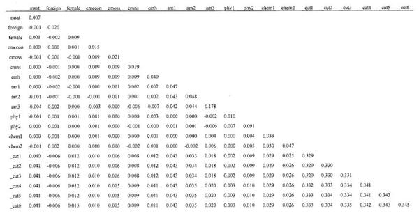
If you type the command
.vce ,
Stata will report
as shown in Figure 4. We need the section of this matrix shown in Part A of Table 6. Use equation (5) to estimate the standard errors of the estimates of the cutoff points and complete Part B of Table 6 and compares the t-ratios with the values reported by Butler, et al. (and shown in the last column 4 of Table 6). Are you satisfied that we have been able to come reasonably close to the results reported in the article?
Stata estimate of the variance-covariance matrix.
Calculation of the t-ratios for the cutoff estimates.
Part A. Relevant portion of the variance-covariance matrix.
_cut1
_cut2
_cut3
_cut4
_cut5
_cut6
_cut1
0.329
_cut2
0.329
0.330
_cut3
0.329
0.330
0.331
_cut4
0.332
0.333
0.334
0.341
_cut5
0.333
0.334
0.334
0.341
0.343
_cut6
0.333
0.334
0.335
0.342
0.343
0.345
Part B. Calculation of the t-ratios (with comparison of values reported in BFS)