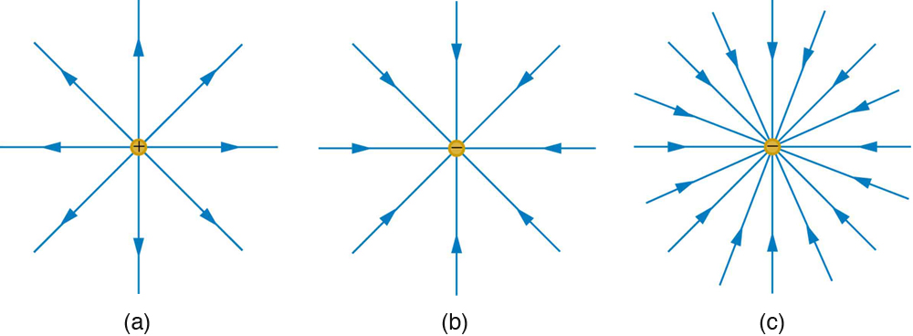
Note that the electric field is defined for a positive test charge
, so that the field lines point away from a positive charge and toward a negative charge. (See
[link] .) The electric field strength is exactly proportional to the number of field lines per unit area, since the magnitude of the electric field for a point charge is
and area is proportional to
. This pictorial representation, in which field lines represent the direction and their closeness (that is, their areal density or the number of lines crossing a unit area) represents strength, is used for all fields: electrostatic, gravitational, magnetic, and others.
The electric field surrounding three different point charges. (a) A positive charge. (b) A negative charge of equal magnitude. (c) A larger negative charge.
In many situations, there are multiple charges. The total electric field created by multiple charges is the vector sum of the individual fields created by each charge. The following example shows how to add electric field vectors.
Adding electric fields
Find the magnitude and direction of the total electric field due to the two point charges,
and
, at the origin of the coordinate system as shown in
[link] .
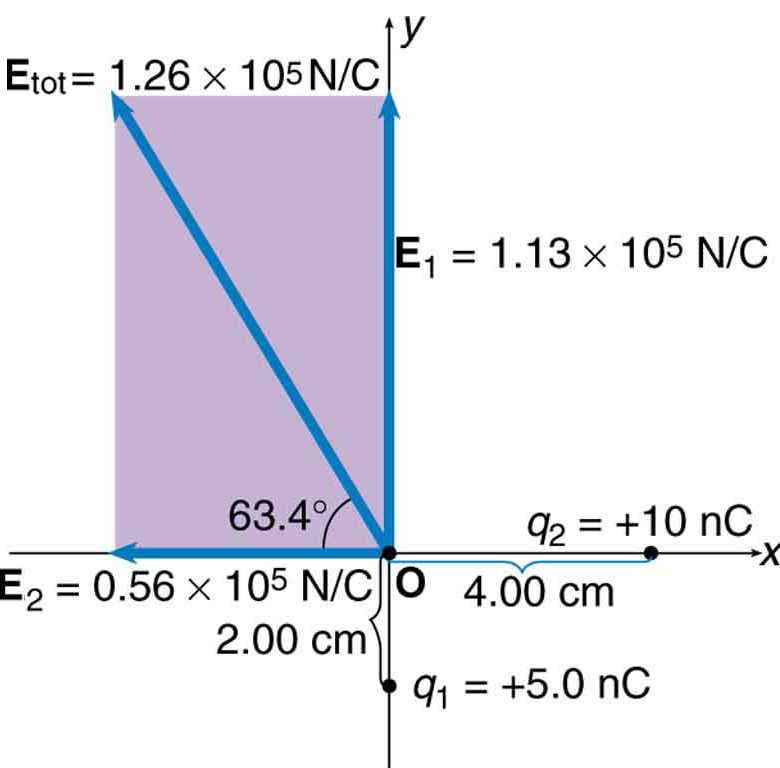
The electric fields
and
at the origin O add to
.
Strategy
Since the electric field is a vector (having magnitude and direction), we add electric fields with the same vector techniques used for other types of vectors. We first must find the electric field due to each charge at the point of interest, which is the origin of the coordinate system (O) in this instance. We pretend that there is a positive test charge,
, at point O, which allows us to determine the direction of the fields
and
. Once those fields are found, the total field can be determined using
vector addition .
Solution
The electric field strength at the origin due to
is labeled
and is calculated:
Similarly,
is
Four digits have been retained in this solution to illustrate that
is exactly twice the magnitude of
. Now arrows are drawn to represent the magnitudes and directions of
and
. (See
[link] .) The direction of the electric field is that of the force on a positive charge so both arrows point directly away from the positive charges that create them. The arrow for
is exactly twice the length of that for
. The arrows form a right triangle in this case and can be added using the Pythagorean theorem. The magnitude of the total field
is
The direction is
or
above the
x -axis.
Discussion
In cases where the electric field vectors to be added are not perpendicular, vector components or graphical techniques can be used. The total electric field found in this example is the total electric field at only one point in space. To find the total electric field due to these two charges over an entire region, the same technique must be repeated for each point in the region. This impossibly lengthy task (there are an infinite number of points in space) can be avoided by calculating the total field at representative points and using some of the unifying features noted next.
Questions & Answers
differentiate between demand and supply
giving examples
In economics, a perfect market refers to a theoretical construct where all participants have perfect information, goods are homogenous, there are no barriers to entry or exit, and prices are determined solely by supply and demand. It's an idealized model used for analysis,
When MP₁ becomes negative, TP start to decline.
Extuples Suppose that the short-run production function of certain cut-flower firm is given by: Q=4KL-0.6K2 - 0.112 •
Where is quantity of cut flower produced, I is labour input and K is fixed capital input (K-5). Determine the average product of lab
Kelo
Extuples Suppose that the short-run production function of certain cut-flower firm is given by: Q=4KL-0.6K2 - 0.112 •
Where is quantity of cut flower produced, I is labour input and K is fixed capital input (K-5). Determine the average product of labour (APL) and marginal product of labour (MPL)
Quantity demanded refers to the specific amount of a good or service that consumers are willing and able to purchase at a give price and within a specific time period. Demand, on the other hand, is a broader concept that encompasses the entire relationship between price and quantity demanded
Ezea
ok
Shukri
how do you save a country economic situation when it's falling apart
Economic growth as an increase in the production and consumption of goods and services within an economy.but
Economic development as a broader concept that encompasses not only economic growth but also social & human well being.
Shukri
production function means
Jabir
What do you think is more important to focus on when considering inequality ?
sir...I just want to ask one question... Define the term contract curve? if you are free please help me to find this answer 🙏
Asui
it is a curve that we get after connecting the pareto optimal combinations of two consumers after their mutually beneficial trade offs
Awais
thank you so much 👍 sir
Asui
In economics, the contract curve refers to the set of points in an Edgeworth box diagram where both parties involved in a trade cannot be made better off without making one of them worse off. It represents the Pareto efficient allocations of goods between two individuals or entities, where neither p
Cornelius
In economics, the contract curve refers to the set of points in an Edgeworth box diagram where both parties involved in a trade cannot be made better off without making one of them worse off. It represents the Pareto efficient allocations of goods between two individuals or entities,
Cornelius
Suppose a consumer consuming two commodities X and Y has
The following utility function u=X0.4 Y0.6. If the price of the X and Y are 2 and 3 respectively and income Constraint is birr 50.
A,Calculate quantities of x and y which maximize utility.
B,Calculate value of Lagrange multiplier.
C,Calculate quantities of X and Y consumed with a given price.
D,alculate optimum level of output .
the market for lemon has 10 potential consumers, each having an individual demand curve p=101-10Qi, where p is price in dollar's per cup and Qi is the number of cups demanded per week by the i th consumer.Find the market demand curve using algebra. Draw an individual demand curve and the market dema
suppose the production function is given by ( L, K)=L¼K¾.assuming capital is fixed find APL and MPL. consider the following short run production function:Q=6L²-0.4L³ a) find the value of L that maximizes output b)find the value of L that maximizes marginal product