Introduction to vector spaces

For much of its history, signal processing has focused on signals produced by physical systems. Many natural and man-made systems can be modeled as linear. Thus, it is natural to consider signal models that complement this kind of linear structure. This notion has been incorporated into modern signal processing by modeling signals as vectors living in an appropriate vector space . This captures the linear structure that we often desire, namely that if we add two signals together then we obtain a new, physically meaningful signal. Moreover, vector spaces allow us to apply intuitions and tools from geometry in ${\mathbb{R}}^3$ , such as lengths, distances, and angles, to describe and compare signals of interest. This is useful even when our signals live in high-dimensional or infinite-dimensional spaces.

Throughout this course , we will treat signals as real-valued functions having domains that are either continuous or discrete, and either infinite or finite. These assumptions will be made clear as necessary in each chapter. In this course, we will assume that the reader is relatively comfortable with the key concepts in vector spaces. We now provide only a brief review of some of the key concepts in vector spaces that will be required in developing the theory of compressive sensing (CS). For a more thorough review of vector spaces see this introductory course in Digital Signal Processing .

We will typically be concerned with normed vector spaces , i.e., vector spaces endowed with a norm . In the case of a discrete, finite domain, we can view our signals as vectors in an $N$ -dimensional Euclidean space, denoted by ${\mathbb{R}}^N$ . When dealing with vectors in ${\mathbb{R}}^N$ , we will make frequent use of the ${\ell }_p$ norms, which are defined for $p\in [1,\infty ]$ as

In Euclidean space we can also consider the standard inner product in ${\mathbb{R}}^N$ , which we denote

This inner product leads to the ${\ell }_2$ norm: ${∥x∥}_2=\sqrt{⟨x,x⟩}$ .

In some contexts it is useful to extend the notion of ${\ell }_p$ norms to the case where $p<1$ . In this case, the “norm” defined in [link] fails to satisfy the triangle inequality, so it is actually a quasinorm. We will also make frequent use of the notation ${∥x∥}_0:=\left|\mathrm{supp}\left(x\right)\right|$ , where $\mathrm{supp}\left(x\right)=\{i:x_i\ne 0\}$ denotes the support of $x$ and $\left|\mathrm{supp}\right(x\left)\right|$ denotes the cardinality of $\mathrm{supp}\left(x\right)$ . Note that ${∥·∥}_0$ is not even a quasinorm, but one can easily show that

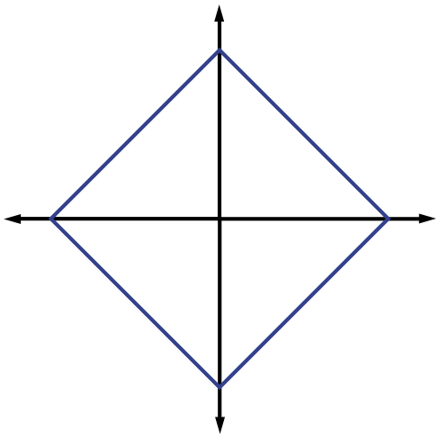
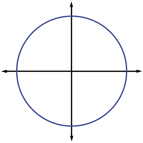
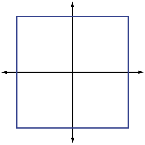
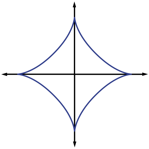
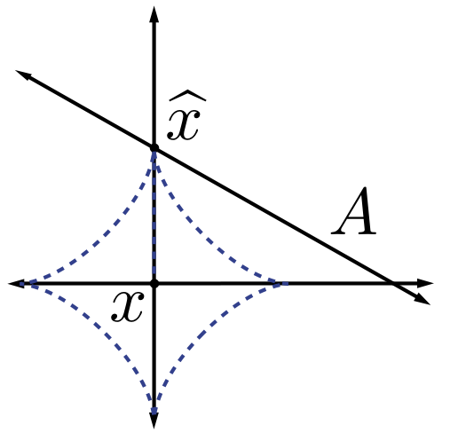
justifying this choice of notation. The ${\ell }_p$ (quasi-)norms have notably different properties for different values of $p$ . To illustrate this, in [link] we show the unit sphere, i.e., $\{x:{∥x∥}_p=1\},$ induced by each of these norms in ${\mathbb{R}}^2$ . Note that for $p<1$ the corresponding unit sphere is nonconvex (reflecting the quasinorm's violation of the triangle inequality).

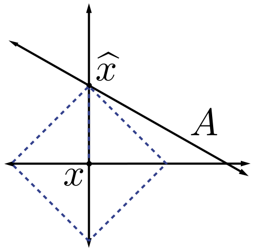
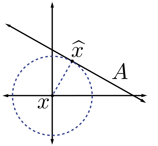
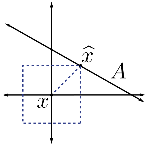
We typically use norms as a measure of the strength of a signal, or the size of an error. For example, suppose we are given a signal $x\in {\mathbb{R}}^2$ and wish to approximate it using a point in a one-dimensional affine space $A$ . If we measure the approximation error using an ${\ell }_p$ norm, then our task is to find the $\widehat{x}\in A$ that minimizes ${∥x,-,\widehat{x}∥}_p$ . The choice of $p$ will have a significant effect on the properties of the resulting approximation error. An example is illustrated in [link] . To compute the closest point in $A$ to $x$ using each ${\ell }_p$ norm, we can imagine growing an ${\ell }_p$ sphere centered on $x$ until it intersects with $A$ . This will be the point $\widehat{x}\in A$ that is closest to $x$ in the corresponding ${\ell }_p$ norm. We observe that larger $p$ tends to spread out the error more evenly among the two coefficients, while smaller $p$ leads to an error that is more unevenly distributed and tends to be sparse. This intuition generalizes to higher dimensions, and plays an important role in the development of CS theory.