Chapter 1: magnetic circuits and magnetic materials  (Page 2/5)

A magnetic circuit with an air gap is shown in Fig.1.2. Air gaps are present for moving elements. The air gap length is sufficiently small. $\phi$ : the flux in the magnetic circuit.

Figure 1.2Magnetic circuit with air gap.

$B_c=\frac{\phi }{A_c}$ (1.7)

$B_g=\frac{\phi }{A_g}$ (1.8)

$F=H_c{l}_c+H_g{l}_g$ (1.9)

$F=\frac{B_c}{\mu }{l}_c+\frac{B_g}{{\mu }_0}g$ (1.10)

$F=\phi (\frac{l_c}{{\mathrm{\mu A}}_c}+\frac{g}{{\mu }_0{A}_g})$ (1.11)

• $R_c$ , $R_g$ : the reluctance of the core and the air gap, respectively,

$R_c=\frac{l_c}{{\mathrm{\mu A}}_c}$ (1.12)

$R_g=\frac{g}{{\mu }_0{A}_g}$ (1.13)

$F=\phi (R_c+R_g)$ (1.14)

$\phi =\frac{F}{R_c+R_g}$ (1.15)

$\phi =\frac{F}{\frac{l_c}{{\mathrm{\mu A}}_c}+\frac{g}{{\mu }_0{A}_g}}$ (1.16)

• In general, for any magnetic circuit of total reluctance $R_{\text{tot}}$ , the flux can be found as

$\phi =\frac{F}{R_{\text{tot}}}$ (1.17)

The permeance P is the inverse of the reluctance

$P_{\text{tot}}=\frac{1}{R_{\text{tot}}}$ (1.18)

• Fig. 1.3: Analogy between electric and magnetic circuits:

Figure 1.3:Analogy between electric and magnetic circuits: (a) electric ckt, (b) magnetic ckt.

• Note that with high material permeability: and thus

$\phi \approx \frac{F}{R_g}=\frac{{\mathrm{F\mu }}_0{A}_g}{g}=\text{Ni}\frac{{\mu }_0{A}_g}{g}$ (1.19)

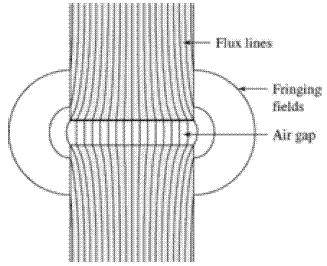
• Fig. 1.4: Fringing effect, effective $A_g$ increased.

Figure 1.4 Air-gap fringing fields.

• In general, magnetic circuits can consist of multiple elements in series and parallel.

$F=\oint \text{Hdl}=\sum _k{F}_k=\sum _k{H}_k{l}_k$ (1.20)

$F={\int }_{s}J\text{.}\text{da}$ (1.21)

$V=\sum _k{R}_k{i}_k$ (1.22)

$\sum _n{i}_n=0$ (1.23)

$\sum _n{\phi }_n=0$ (1.24)

§1.2 Flux Linkage, Inductance, and Energy

• Faraday’s Law:

${\oint }_{c}E\text{.}\text{ds}=-\frac{d}{\text{dt}}{\int }_{s}B\text{.}\text{da}$ (1.25)

• $\lambda$ : the flux linkage of the winding, $\varphi$ : the instantaneous value of a time-varying flux,
• e : the induced voltage at the winding terminals

$\begin{array}{}e=N\frac{\mathrm{d\varphi }}{\text{dt}}=\frac{\mathrm{d\lambda }}{\text{dt}}\\ \lambda =\mathrm{N\varphi }\end{array}$ (1.26)

• L : the inductance (with material of constant permeability), H = Wb-t/A

$L=\frac{\lambda }{i}$ (1.27)

$L=\frac{N^2}{R_{\text{tot}}}$ (1.28)

• The inductance of the winding in Fig. 1.2:

$L=\frac{N^2}{(g/{\mu }_0{A}_g)}=\frac{N^2{\mu }_0{A}_g}{g}$ (1.29)

• Magnetic circuit with more than one windings, Fig. 1.5:

Figure 1.5Magnetic circuit with two windings.

$F=N_1{i}_1+N_2{i}_2$ (1.30)

$\phi =(N_1{i}_1+N_2{i}_2)\frac{{\mu }_0{A}_c}{g}$ (1.31)

${\lambda }_1=N_1\phi =N_1^2(\frac{{\mu }_0{A}_c}{g})i_1+N_1{N}_2(\frac{{\mu }_0{A}_c}{g})i_2$ (1.32)

${\lambda }_1=L_{\text{11}}{i}_1+L_{\text{12}}{i}_2$ (1.33)

$L_{\text{11}}=N_1^2\frac{{\mu }_0{A}_c}{g}$ (1.34)

$L_{\text{12}}=N_1{N}_2\frac{{\mu }_0{A}_c}{g}=L_{\text{21}}$ (1.35)

${\lambda }_2=N_2\phi =N_1{N}_2(\frac{{\mu }_0{A}_c}{g})i_1+N_2^2(\frac{{\mu }_0{A}_c}{g})i_2$ (1.36)

${\lambda }_2=L_{\text{21}}{i}_1+L_{\text{22}}{i}_2$ (1.37)

$L_{\text{22}}=N_2^2\frac{{\mu }_0{A}_c}{g}$ (1.38)

• Induced voltage, power (W = J/s), and stored energy:

$e=\frac{d}{\text{dt}}(\text{Li})$ (1.39)

$e=L\frac{\text{di}}{\text{dt}}+i\frac{\text{dL}}{\text{dt}}$ (1.40)

$p=\text{ie}=i\frac{\mathrm{d\lambda }}{\text{dt}}$ (1.41)

$\mathrm{\Delta W}={\int }_{t_1}^{t_2}\text{pdt}={\int }_{{\lambda }_1}^{{\lambda }_2}\text{id}\lambda$ (1.42)

$\mathrm{\Delta W}={\int }_{{\lambda }_1}^{{\lambda }_2}\text{id}\lambda ={\int }_{{\lambda }_1}^{{\lambda }_2}\frac{\lambda }{L}\mathrm{d\lambda }=\frac{1}{\mathrm{2L}}({\lambda }_2^2-{\lambda }_1^1)$ (1.43)

$W=\frac{1}{\mathrm{2L}}{\lambda }^2=\frac{L}{2}{i}^2$ (1.44)

§1.3 Properties of Magnetic Materials

• The importance of magnetic materials is twofold:

• Magnetic materials are used to obtain large magnetic flux densities with relatively low levels of magnetizing force.
• Magnetic materials can be used to constrain and direct magnetic fields in well defined paths.

• Ferromagnetic materials, typically composed of iron and alloys of iron with cobalt, tungsten, nickel, aluminum, and other metals, are by far the most common magnetic materials.

• They are found to be composed of a large number of domains.
• When unmagnetized, the domain magnetic moments are randomly oriented.
• When an external magnetizing force is applied, the domain magnetic moments tend to align with the applied magnetic field until all the magnetic moments are aligned with the applied field, and the material is said to be fully saturated.
• When the applied field is reduced to zero, the magnetic dipole moments will no longer be totally random in their orientation and will retain a net magnetization component along the applied field direction.