3.7 Solving linear constant coefficient differential equations  (Page 2/2)

Consider the decay model in which a quantity of an unstable isotope decreases at a rate proportional to the quanity of unstable isotope remaining. Thus, the decay of the isotope is modeled by the first order linear constant coefficient differential equation

where $r$ is some real rate. This differential equation could easily be solved through straightforward integration. However, the methods described above will be used instead. Note that the forcing function is zero, so only a homogenous solution is needed. It is easy to see that the characteristic polynomial is $\lambda +r=0$ , so there is one root ${\lambda }_1=r$ . Thus the solution is of the form

Given a rate and an initial condition, this can be applied to a specific situation. For instance, we know that carbon-14 decays at a rate of approximately $r=1.21\mathrm{x}{10}^{-4}$ ${\mathrm{year}}^{-1}$ , and if we normalize the natural concentration of carbon-14 to $x\left(0\right)=1$ the solution becomes $x\left(t\right)=e^{-1.21\mathrm{x}{10}^{-4}t}$ . Knowledge of this curve would be useful for radioisotope based dating.

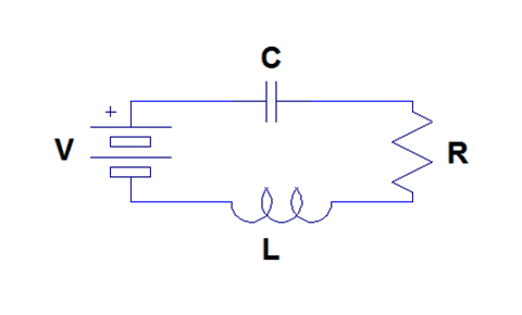
Consider the series RLC circuit shown in [link] . This system can be modeled using differential equations. We can use the voltage equations for each circuit element and Kirchoff's voltage law to write a second order linear constant coefficient differential equation describing the charge on the capacitor.

The voltage across the battery is simply $V$ . The voltage across the capacitor is $\frac{1}{C}q$ . The voltage across the resistor is $R\frac{dq}{dt}$ . Finally, the voltage across the inductor is $L\frac{d^{2}q}{d{t}^2}$ . Therefore, by Kirchoff's voltage law, it follows that

First, the homogeneous solution is found. It is easy to see that the characteristic polynomial is $L{\lambda }^2+R\lambda +\frac{1}{C}=0$ . Therefore, the two roots are ${\lambda }_1=\frac{-R-\sqrt{R^2-\frac{4L}{C}}}{2L}$ and ${\lambda }_2=\frac{-R+\sqrt{R^2-\frac{4L}{C}}}{2L}$ . Often, these are stated in terms of the attenuation factor $\alpha =\frac{R}{2}\sqrt{\frac{C}{L}}$ and the resonant frequency ${\omega }_0=\frac{1}{\sqrt{LC}}$ . Thus, ${\lambda }_1=-\alpha -\sqrt{{\alpha }^2-{\omega }_0^2}$ and ${\lambda }_2=-\alpha +\sqrt{{\alpha }^2-{\omega }_0^2}$ .

Thus, the homogeneous equation is of the form

It turns out that the response to the constant voltage source forcing function is a constant, so

Hence, the general solution is

where $c_1$ and $c_2$ depend on the initial conditions. The system demonstrates a rich array of behaviors based on the relative values of $\alpha$ and ${\omega }_0$ , which the reader is encouraged to explore.