

| << Chapter < Page | Chapter >> Page > |
This can be rewritten using the identity in [link] to produce
Rewriting as the sum of its (positive) average value and the variation about this average yields
Thus,
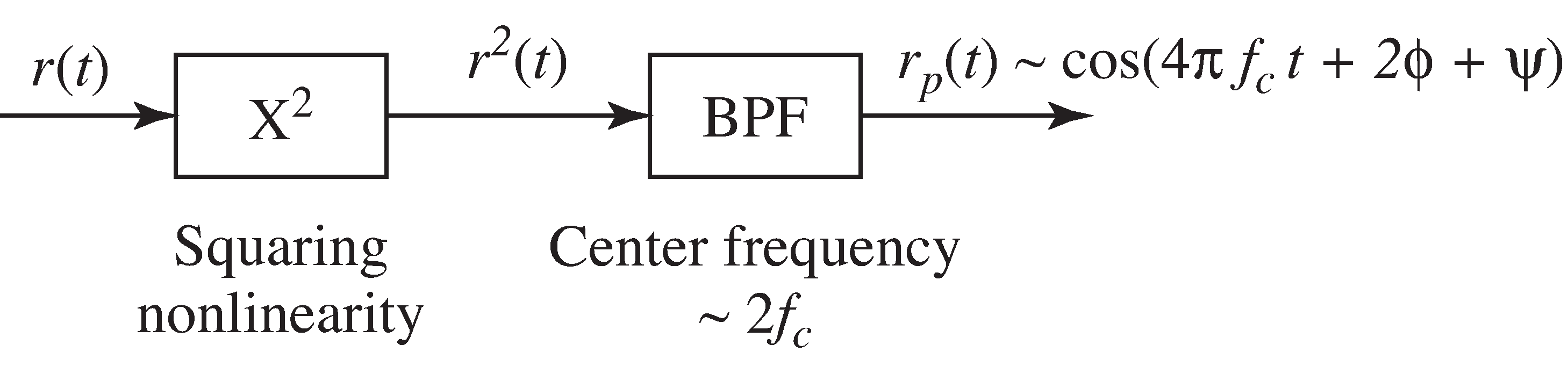
A narrow bandpass filter centered near passes the pure cosine term in and suppresses the DC component, the (presumably) lowpass , and the upconverted . The output of the bandpass filter is approximately
where is the phase shift added by the BPF at frequency . Since is known at the receiver, can be used to find the frequency and phase of the carrier.Of course, the primary component in is at twice the frequency of thecarrier, the phase is twice the original unknown phase, and it is necessary to take into account. Thus some extra bookkeeping is needed.The amplitude of undulates slowly as changes.
The following M
atlab code carries out the
preprocessing of
[link] .
First, run
pulrecsig.m to generate
the suppressed carrier signal
rsc .
label=cod:pllpreprocess]
 r=rsc;                            % r generated with suppressed carrier
q=r.^2;                           % square nonlinearityfl=500; ff=[0 .38 .39 .41 .42 1];  % BPF center frequency at .4fa=[0 0 1 1 0 0];                 % which is twice f_0h=firpm(fl,ff,fa);                % BPF design via firpm
rp=filter(h,1,q);                 % filter to give preprocessed r

pllpreprocess.m
(download file)
Then the phase and frequency of
rp can be found directly by using the FFT.
% recover unknown freq and phase using FFT
fftrBPF=fft(rp);                      % spectrum of rBPF[m,imax]=max(abs(fftrBPF(1:end/2)));  % find frequency of max peakssf=(0:length(rp))/(Ts*length(rp));   % frequency vector
freqS=ssf(imax)                       % freq at the peakphasep=angle(fftrBPF(imax));          % phase at the peak
[IR,f]=freqz(h,1,length(rp),1/Ts);    % frequency response of filter
[mi,im]=min(abs(f-freqS));            % at freq where peak occurs
phaseBPF=angle(IR(im));               % angle of BPF at peak freqphaseS=mod(phasep-phaseBPF,pi)        % estimated angle
Observe that both
freqS and
phaseS are twice the
nominal values of
fc and
phoff , though there may be
a
ambiguity (as will occur in any phase estimation).
The intent of this section is to clearly depict the problem of recovering the frequency and phase of the carrier even whenit is buried within the data modulated signal. The method used to solve the problem (application of the FFT)is not common, primarily because of the numerical complexity. Most practical receivers use some kind of adaptive elementto iteratively locate and track the frequency and phase of the carrier. Such elements are explored in the remainder of this chapter.
Notification Switch
Would you like to follow the 'Software receiver design' conversation and receive update notifications?

|
|

|
|

|
|

|
|

|
|

|
|

|
|

|
|

|
|
|
|