

| << Chapter < Page | Chapter >> Page > |
Lecture #6:
CONTINUOUS TIME FOURIER TRANSFORM (CTFT)
Motivation:
Outline:
– Fourier transform of the unit step function
– Fourier transform of causal sinusoids
– Fourier transform of rectangular pulse — the sinc function
– Fourier transform of triangular pulse
Example — How to filter the ECG?
The recorded activity from the surface of the chest includes the electrical activity of the heart plus extraneous signals or “noise.” How can we design a filter that will reduce the noise?
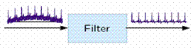
It is most effective to compute the frequency content of the recorded signal and to identify those components that are due to the electrical activity of the heart and those that are noise. Then the filter can be designed rationally. This is one of many motivations for understanding the Fourier transform.
I. THE CONTINUOUS TIME FOURIER TRANSFORM (CTFT)
1/ Definition
The continuous time Fourier transform of x(t) is defined as
and the inverse transform is defined as
2/ Relation of Fourier and Laplace Transforms
The bilateral Laplace transform is defined by the analysis formula
and the inverse transform is defined by the synthesis formula
Now if the jω axis is in the region of convergence of X(s), then we can substitute s = jω = j2πf into both relations to obtain
3/ Form of the Fourier transform
Finally, by canceling j2π and changing the variable of integration from j2πf to f we obtain
It is clumsy to write X(j2πf). Therefore, from this now on, we rewrite the function X(j2πf) described above as in a simpler form X(f) such that the transform pair would be symmetrical.
X(j2πf) Þ X(f)
The new Fourier transform pair will be in the form
4/ Notation
Notation for the Fourier transform varies appreciably from text to text and in different disciplines. Another common notation is to define the Fourier transform in terms of jω as follows
Differences in notation are largely a matter of taste and different notations result in different locations of factors of 2π. The notation we use minimizes the number of factors of 2π that appear in the expressions we will use in this subject and makes the duality of the Fourier transform with its inverse more transparent.
Notification Switch
Would you like to follow the 'Signals and systems' conversation and receive update notifications?

|
|

|
|

|
|

|
|

|
|

|
|

|
|

|
|

|
|

|