

| << Chapter < Page | Chapter >> Page > |
This section develops the properties of the Butterworth filter which has as its basic concept a Taylor's seriesapproximation to the desired frequency response. The measure of the approximation is the number of terms in the Taylor's seriesexpansion of the actual frequency response that can be made equal to those of the desired frequency response. The optimal or bestsolution will have the maximum number of terms equal. The Taylor's series is a power series expansion of a function in theform of
where
with the coefficients of the Taylor's series being proportional to the various order derivatives of evaluated at . A basic characteristic of this approach is that the approximation is all performed at onepoint, i.e., at one frequency. The ability of this approach to give good results over a range of frequencies depends on the analyticproperties of the response.
The general form for the squared-magnitude response is an even function of and, therefore, is a function of expressed as
In order to obtain a solution that is a lowpass filter, the Taylor's series expansion is performed around , requiring that and that , (i.e., , , and ). This is written as
Combining [link] and [link] gives
The best Taylor's approximation requires that and the desired ideal response have as many terms as possible equal in theirTaylor's series expansion at a given frequency. For a lowpass filter, the expansion is around , and this requires have as few low-order terms as possible. This is achieved by setting
Because the ideal response in the passband is a constant, the Taylor's series approximation is often called “maximally flat".
[link] states that the numerator of the transfer function may be chosen arbitrarily. Then by setting the denominatorcoefficients of FF(s) equal to the numerator coefficients plus one higher-order term, an optimal Taylor's series approximation isachieved [link] .
Since the numerator is arbitrary, its coefficients can be chosen for a Taylor's approximation to zero at . This is accomplished by setting and all other d's equal zero. The resulting magnitude-squared function is [link]
The value of the constant determines at which value of the transition of passband to stopband occurs. For this development, it is normalized to , which causes the transition to occur at . This gives the simple form for what is called the Butterworth filter
This approximation is sometimes called “maximally flat" at both and , since it is simultaneously a Taylor's series approximation to unity at and to zero at . A graph of the resulting frequency response function is shown in [link] for several .
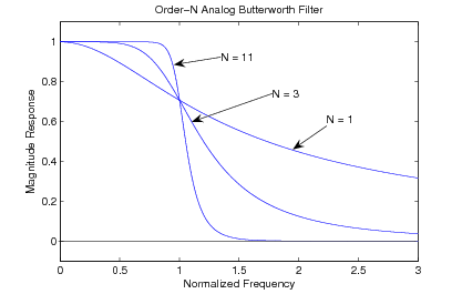
The characteristics of the normalized Butterworth filter frequency response are:
Notification Switch
Would you like to follow the 'Filter design - sidney burrus style' conversation and receive update notifications?

|
|

|
|

|
|

|
|

|
|
|
|
|

|
|
|
|
|
|
|
|

|