

| << Chapter < Page | Chapter >> Page > |
[link] illustrates the idea of economies of scale, showing the average cost of producing an alarm clock falling as the quantity of output rises. For a small-sized factory like S, with an output level of 1,000, the average cost of production is $12 per alarm clock. For a medium-sized factory like M, with an output level of 2,000, the average cost of production falls to $8 per alarm clock. For a large factory like L, with an output of 5,000, the average cost of production declines still further to $4 per alarm clock.
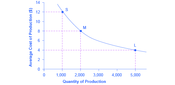
The average cost curve in [link] may appear similar to the average cost curves presented earlier in this chapter, although it is downward-sloping rather than U-shaped. But there is one major difference. The economies of scale curve is a long-run average cost curve, because it allows all factors of production to change. The short-run average cost curves presented earlier in this chapter assumed the existence of fixed costs, and only variable costs were allowed to change.
One prominent example of economies of scale occurs in the chemical industry. Chemical plants have a lot of pipes. The cost of the materials for producing a pipe is related to the circumference of the pipe and its length. However, the volume of chemicals that can flow through a pipe is determined by the cross-section area of the pipe. The calculations in [link] show that a pipe which uses twice as much material to make (as shown by the circumference of the pipe doubling) can actually carry four times the volume of chemicals because the cross-section area of the pipe rises by a factor of four (as shown in the Area column).
| Circumference ( ) | Area ( ) | |
|---|---|---|
| 4-inch pipe | 12.5 inches | 12.5 square inches |
| 8-inch pipe | 25.1 inches | 50.2 square inches |
| 16-inch pipe | 50.2 inches | 201.1 square inches |
A doubling of the cost of producing the pipe allows the chemical firm to process four times as much material. This pattern is a major reason for economies of scale in chemical production, which uses a large quantity of pipes. Of course, economies of scale in a chemical plant are more complex than this simple calculation suggests. But the chemical engineers who design these plants have long used what they call the “six-tenths rule,” a rule of thumb which holds that increasing the quantity produced in a chemical plant by a certain percentage will increase total cost by only six-tenths as much.
While in the short run firms are limited to operating on a single average cost curve (corresponding to the level of fixed costs they have chosen), in the long run when all costs are variable, they can choose to operate on any average cost curve. Thus, the long-run average cost (LRAC) curve is actually based on a group of short-run average cost (SRAC) curves , each of which represents one specific level of fixed costs. More precisely, the long-run average cost curve will be the least expensive average cost curve for any level of output. [link] shows how the long-run average cost curve is built from a group of short-run average cost curves. Five short-run-average cost curves appear on the diagram. Each SRAC curve represents a different level of fixed costs. For example, you can imagine SRAC 1 as a small factory, SRAC 2 as a medium factory, SRAC 3 as a large factory, and SRAC 4 and SRAC 5 as very large and ultra-large. Although this diagram shows only five SRAC curves, presumably there are an infinite number of other SRAC curves between the ones that are shown. This family of short-run average cost curves can be thought of as representing different choices for a firm that is planning its level of investment in fixed cost physical capital—knowing that different choices about capital investment in the present will cause it to end up with different short-run average cost curves in the future.
Notification Switch
Would you like to follow the 'Principles of economics' conversation and receive update notifications?

|
|
|
|
|

|
|

|
|

|
|

|
|

|
|

|
|

|
|

|
|

|
|

|