<< Chapter < Page Chapter >> Page >
By the end of this section, you will be able to:
  • Describe the physical factors that lead to deviations from ideal gas behavior
  • Explain how these factors are represented in the van der Waals equation
  • Define compressibility (Z) and describe how its variation with pressure reflects non-ideal behavior
  • Quantify non-ideal behavior by comparing computations of gas properties using the ideal gas law and the van der Waals equation

Thus far, the ideal gas law, PV = nRT , has been applied to a variety of different types of problems, ranging from reaction stoichiometry and empirical and molecular formula problems to determining the density and molar mass of a gas. As mentioned in the previous modules of this chapter, however, the behavior of a gas is often non-ideal, meaning that the observed relationships between its pressure, volume, and temperature are not accurately described by the gas laws. In this section, the reasons for these deviations from ideal gas behavior are considered.

One way in which the accuracy of PV = nRT can be judged is by comparing the actual volume of 1 mole of gas (its molar volume, V m ) to the molar volume of an ideal gas at the same temperature and pressure. This ratio is called the compressibility factor (Z)    with:

Z = molar volume of gas at same T and P molar volume of ideal gas at same T and P = ( P V m R T ) measured

Ideal gas behavior is therefore indicated when this ratio is equal to 1, and any deviation from 1 is an indication of non-ideal behavior. [link] shows plots of Z over a large pressure range for several common gases.

A graph is shown. The horizontal axis is labeled, “P ( a t m ).” Its scale begins at zero with markings provided by multiples of 200 up to 1000. The vertical axis is labeled, “Z le( k P a ).” This scale begins at zero and includes multiples of 0.5 up to 2.0. Six curves are drawn of varying colors. One of these curves is a horizontal, light purple line extending right from 1.0 k P a on the vertical axis, which is labeled “Ideal gas.” The region of the graph beneath this line is shaded tan. The remaining curves also start at the same point on the vertical axis. An orange line extends to the upper right corner of the graph, reaching a value of approximately 1.7 k P a at 1000 a t m. This orange curve is labeled, “H subscript 2.” A blue curve dips below the horizontal ideal gas line initially, then increases to cross the line just past 200 a t m. This curve reaches a value of nearly 2.0 k P a at about 800 a t m. This curve is labeled, “N subscript 2.” A red curve dips below the horizontal ideal gas line initially, then increases to cross the line just past 400 a t m. This curve reaches a value of nearly 1.5 k P a at about 750 a t m. This curve is labeled, “O subscript 2.” A purple curve dips below the horizontal ideal gas line, dipping even lower than the O subscript 2 curve initially, then increases to cross the ideal gas line at about 400 a t m. This curve reaches a value of nearly 2.0 k P a at about 850 a t m. This curve is labeled, “C H subscript 4.” A yellow curve dips below the horizontal ideal gas line, dipping lower than the other curves to a minimum of about 0.4 k P a at about 0.75 a t m, then increases to cross the ideal gas line at about 500 a t m. This curve reaches a value of about 1.6 k P a at about 900 a t m. This curve is labeled, “C O subscript 2.”
A graph of the compressibility factor (Z) vs. pressure shows that gases can exhibit significant deviations from the behavior predicted by the ideal gas law.

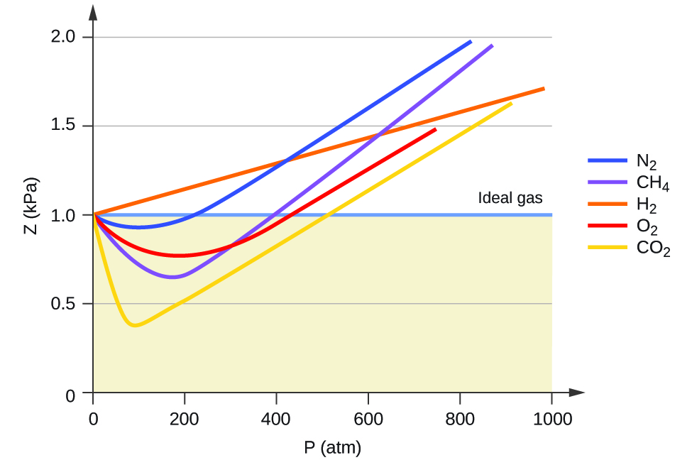
As is apparent from [link] , the ideal gas law does not describe gas behavior well at relatively high pressures. To determine why this is, consider the differences between real gas properties and what is expected of a hypothetical ideal gas.

Particles of a hypothetical ideal gas have no significant volume and do not attract or repel each other. In general, real gases approximate this behavior at relatively low pressures and high temperatures. However, at high pressures, the molecules of a gas are crowded closer together, and the amount of empty space between the molecules is reduced. At these higher pressures, the volume of the gas molecules themselves becomes appreciable relative to the total volume occupied by the gas ( [link] ). The gas therefore becomes less compressible at these high pressures, and although its volume continues to decrease with increasing pressure, this decrease is not proportional as predicted by Boyle’s law.

This figure includes three diagrams. In a, a cylinder with 9 purple spheres with trails indicating motion are shown. Above the cylinder, the label, “Particles ideal gas,” is connected to two of the spheres with line segments extending into the square. The label “Assumes” is beneath the square. In b, a cylinder and piston is shown. A relatively small open space is shaded lavender with 9 purple spheres packed close together. No motion trails are present on the spheres. Above the piston, a downward arrow labeled “Pressure” is directed toward the enclosed area. In c, the cylinder is exactly the same as the first, but the number of molecules has doubled.
Raising the pressure of a gas increases the fraction of its volume that is occupied by the gas molecules and makes the gas less compressible.

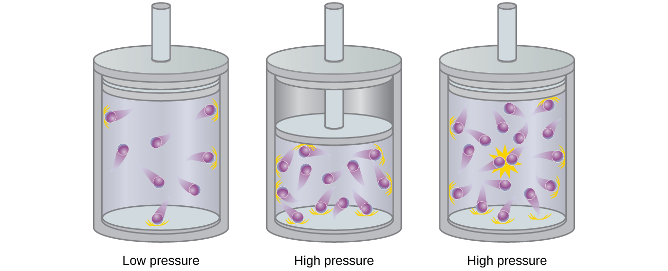
At relatively low pressures, gas molecules have practically no attraction for one another because they are (on average) so far apart, and they behave almost like particles of an ideal gas. At higher pressures, however, the force of attraction is also no longer insignificant. This force pulls the molecules a little closer together, slightly decreasing the pressure (if the volume is constant) or decreasing the volume (at constant pressure) ( [link] ). This change is more pronounced at low temperatures because the molecules have lower KE relative to the attractive forces, and so they are less effective in overcoming these attractions after colliding with one another.

Questions & Answers

how do you get the 2/50
Abba Reply
number of sport play by 50 student construct discrete data
Aminu Reply
width of the frangebany leaves on how to write a introduction
Theresa Reply
Solve the mean of variance
Veronica Reply
Step 1: Find the mean. To find the mean, add up all the scores, then divide them by the number of scores. ... Step 2: Find each score's deviation from the mean. ... Step 3: Square each deviation from the mean. ... Step 4: Find the sum of squares. ... Step 5: Divide the sum of squares by n – 1 or N.
kenneth
what is error
Yakuba Reply
Is mistake done to something
Vutshila
Hy
anas
hy
What is the life teble
anas
hy
Jibrin
statistics is the analyzing of data
Tajudeen Reply
what is statics?
Zelalem Reply
how do you calculate mean
Gloria Reply
diveving the sum if all values
Shaynaynay
let A1,A2 and A3 events be independent,show that (A1)^c, (A2)^c and (A3)^c are independent?
Fisaye Reply
what is statistics
Akhisani Reply
data collected all over the world
Shaynaynay
construct a less than and more than table
Imad Reply
The sample of 16 students is taken. The average age in the sample was 22 years with astandard deviation of 6 years. Construct a 95% confidence interval for the age of the population.
Aschalew Reply
Bhartdarshan' is an internet-based travel agency wherein customer can see videos of the cities they plant to visit. The number of hits daily is a normally distributed random variable with a mean of 10,000 and a standard deviation of 2,400 a. what is the probability of getting more than 12,000 hits? b. what is the probability of getting fewer than 9,000 hits?
Akshay Reply
Bhartdarshan'is an internet-based travel agency wherein customer can see videos of the cities they plan to visit. The number of hits daily is a normally distributed random variable with a mean of 10,000 and a standard deviation of 2,400. a. What is the probability of getting more than 12,000 hits
Akshay
1
Bright
Sorry i want to learn more about this question
Bright
Someone help
Bright
a= 0.20233 b=0.3384
Sufiyan
a
Shaynaynay
How do I interpret level of significance?
Mohd Reply
It depends on your business problem or in Machine Learning you could use ROC- AUC cruve to decide the threshold value
Shivam
how skewness and kurtosis are used in statistics
Owen Reply
yes what is it
Taneeya
Got questions? Join the online conversation and get instant answers!
Jobilize.com Reply
Practice Key Terms 2

Get Jobilize Job Search Mobile App in your pocket Now!

Get it on Google Play Download on the App Store Now


Source:  OpenStax, Chemistry. OpenStax CNX. May 20, 2015 Download for free at http://legacy.cnx.org/content/col11760/1.9
Google Play and the Google Play logo are trademarks of Google Inc.

Notification Switch

Would you like to follow the 'Chemistry' conversation and receive update notifications?

Ask