

| << Chapter < Page | Chapter >> Page > |
In the diagram in [link] , y 0 – ŷ 0 = ε 0 is the residual for the point shown. Here the point lies above the line and the residual is positive.
ε = the Greek letter epsilon
For each data point, you can calculate the residuals or errors, y i - ŷ i = ε i for i = 1, 2, 3, ..., 11.
Each | ε | is a vertical distance.
For the example about the third exam scores and the final exam scores for the 11 statistics students, there are 11 data points. Therefore, there are 11 ε values. If yousquare each ε and add, you get
This is called the Sum of Squared Errors (SSE) .
Using calculus, you can determine the values of a and b that make the SSE a minimum. When you make the SSE a minimum, you have determined the points that are on the line of best fit. It turns out thatthe line of best fit has the equation:
where and .
The sample means of the x values and the y values are and , respectively. The best fit line always passes through the point .
The slope b can be written as where s y = the standard deviation of the y values and s x = the standard deviation of the x values. r is the correlation coefficient, which is discussed in the next section.
The process of fitting the best-fit line is called linear regression . The idea behind finding the best-fit line is based on the assumption that the data are scattered about a straight line. The criteria for the best fit line is that the sum of the squared errors (SSE) is minimized, that is, made as small as possible. Any other line you might choose would have a higher SSE than the best fit line. This best fit line is called the least-squares regression line .
Computer spreadsheets, statistical software, and many calculators can quickly calculate the best-fit line and create the graphs. The calculations tend to be tedious if done by hand. Instructions to use the TI-83, TI-83+, and TI-84+ calculators to find the best-fit line and create a scatterplot are shown at the end of this section.
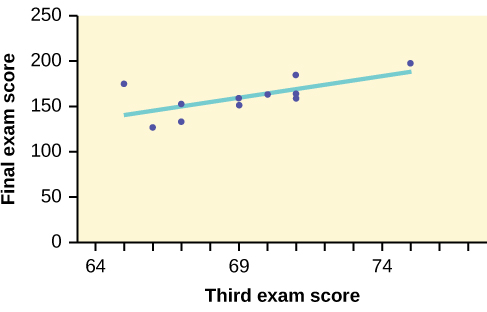
The least squares regression line (best-fit line) for the third-exam/final-exam example has the equation:
Remember, it is always important to plot a scatter diagram first. If the scatter plot indicates that there is a linear relationship between the variables, then it is reasonable to use a best fit line to make predictions for y given x within the domain of x -values in the sample data, but not necessarily for x -values outside that domain. You could use the line to predict the final exam score for a student who earned a grade of 73 on the third exam. You should NOT use the line to predict the final exam score for a student who earned a grade of 50 on the third exam, because 50 is not within the domain of the x -values in the sample data, which are between 65 and 75.
The slope of the line, b , describes how changes in the variables are related. It is important to interpret the slope of the line in the context of the situation represented by the data. You should be able to write a sentence interpreting the slope in plain English.
Notification Switch
Would you like to follow the 'Introductory statistics' conversation and receive update notifications?

|
|
|
|
|

|
|

|
|

|
|

|
|
|
|
|

|
|

|
|

|
|
|
|
|
|
|