<< Chapter < Page Chapter >> Page >

Formula review

s x = f m 2 n x ¯ 2 where s x =  sample standard deviation x ¯  = sample mean

Use the following information to answer the next two exercises : The following data are the distances between 20 retail stores and a large distribution center. The distances are in miles.
29; 37; 38; 40; 58; 67; 68; 69; 76; 86; 87; 95; 96; 96; 99; 106; 112; 127; 145; 150

Use a graphing calculator or computer to find the standard deviation and round to the nearest tenth.

s = 34.5

Got questions? Get instant answers now!

Find the value that is one standard deviation below the mean.

Got questions? Get instant answers now!

Two baseball players, Fredo and Karl, on different teams wanted to find out who had the higher batting average when compared to his team. Which baseball player had the higher batting average when compared to his team?

Baseball Player Batting Average Team Batting Average Team Standard Deviation
Fredo 0.158 0.166 0.012
Karl 0.177 0.189 0.015

For Fredo: z = 0.158  –  0.166 0.012 = –0.67

For Karl: z = 0.177  –  0.189 0.015 = –0.8

Fredo’s z -score of –0.67 is higher than Karl’s z -score of –0.8. For batting average, higher values are better, so Fredo has a better batting average compared to his team.

Got questions? Get instant answers now!

Use [link] to find the value that is three standard deviations:

  • above the mean
  • below the mean
Got questions? Get instant answers now!


Find the standard deviation for the following frequency tables using the formula. Check the calculations with the TI 83/84 .

Find the standard deviation for the following frequency tables using the formula. Check the calculations with the TI 83/84.

  1. Grade Frequency
    49.5–59.5 2
    59.5–69.5 3
    69.5–79.5 8
    79.5–89.5 12
    89.5–99.5 5
  2. Daily Low Temperature Frequency
    49.5–59.5 53
    59.5–69.5 32
    69.5–79.5 15
    79.5–89.5 1
    89.5–99.5 0
  3. Points per Game Frequency
    49.5–59.5 14
    59.5–69.5 32
    69.5–79.5 15
    79.5–89.5 23
    89.5–99.5 2
  1. s x = f m 2 n x ¯ 2 = 193157.45 30 79.5 2 = 10.88
  2. s x = f m 2 n x ¯ 2 = 380945.3 101 60.94 2 = 7.62
  3. s x = f m 2 n x ¯ 2 = 440051.5 86 70.66 2 = 11.14
Got questions? Get instant answers now!

Bringing it together

Twenty-five randomly selected students were asked the number of movies they watched the previous week. The results are as follows:

# of movies Frequency
0 5
1 9
2 6
3 4
4 1
  1. Find the sample mean x .
  2. Find the approximate sample standard deviation, s .
  1. 1.48
  2. 1.12
Got questions? Get instant answers now!

Forty randomly selected students were asked the number of pairs of sneakers they owned. Let X = the number of pairs of sneakers owned. The results are as follows:

X Frequency
1 2
2 5
3 8
4 12
5 12
6 0
7 1
  1. Find the sample mean x
  2. Find the sample standard deviation, s
  3. Construct a histogram of the data.
  4. Complete the columns of the chart.
  5. Find the first quartile.
  6. Find the median.
  7. Find the third quartile.
  8. Construct a box plot of the data.
  9. What percent of the students owned at least five pairs?
  10. Find the 40 th percentile.
  11. Find the 90 th percentile.
  12. Construct a line graph of the data
  13. Construct a stemplot of the data
Got questions? Get instant answers now!

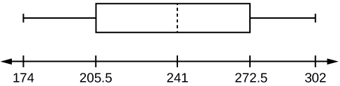
Following are the published weights (in pounds) of all of the team members of the San Francisco 49ers from a previous year.

177; 205; 210; 210; 232; 205; 185; 185; 178; 210; 206; 212; 184; 174; 185; 242; 188; 212; 215; 247; 241; 223; 220; 260; 245; 259; 278; 270; 280; 295; 275; 285; 290; 272; 273; 280; 285; 286; 200; 215; 185; 230; 250; 241; 190; 260; 250; 302; 265; 290; 276; 228; 265

  1. Organize the data from smallest to largest value.
  2. Find the median.
  3. Find the first quartile.
  4. Find the third quartile.
  5. Construct a box plot of the data.
  6. The middle 50% of the weights are from _______ to _______.
  7. If our population were all professional football players, would the above data be a sample of weights or the population of weights? Why?
  8. If our population included every team member who ever played for the San Francisco 49ers, would the above data be a sample of weights or the population of weights? Why?
  9. Assume the population was the San Francisco 49ers. Find:
    1. the population mean, μ .
    2. the population standard deviation, σ .
    3. the weight that is two standard deviations below the mean.
    4. When Steve Young, quarterback, played football, he weighed 205 pounds. How many standard deviations above or below the mean was he?
  10. That same year, the mean weight for the Dallas Cowboys was 240.08 pounds with a standard deviation of 44.38 pounds. Emmit Smith weighed in at 209 pounds. With respect to his team, who was lighter, Smith or Young? How did you determine your answer?
  1. 174; 177; 178; 184; 185; 185; 185; 185; 188; 190; 200; 205; 205; 206; 210; 210; 210; 212; 212; 215; 215; 220; 223; 228; 230; 232; 241; 241; 242; 245; 247; 250; 250; 259; 260; 260; 265; 265; 270; 272; 273; 275; 276; 278; 280; 280; 285; 285; 286; 290; 290; 295; 302
  2. 241
  3. 205.5
  4. 272.5
  5. A box plot with a whisker between 174 and 205.5, a solid line at 205.5, a dashed line at 241, a solid line at 272.5, and a whisker between 272.5 and 302.
  6. 205.5, 272.5
  7. sample
  8. population
    1. 236.34
    2. 37.50
    3. 161.34
    4. 0.84 std. dev. below the mean
  9. Young
Got questions? Get instant answers now!

Get Jobilize Job Search Mobile App in your pocket Now!

Get it on Google Play Download on the App Store Now


Source:  OpenStax, Introductory statistics. OpenStax CNX. May 06, 2016 Download for free at http://legacy.cnx.org/content/col11562/1.18
Google Play and the Google Play logo are trademarks of Google Inc.

Notification Switch

Would you like to follow the 'Introductory statistics' conversation and receive update notifications?

Ask