<< Chapter < Page Chapter >> Page >
Data
x y x y
1915 10.1 1969 36.7
1926 17.7 1975 49.3
1935 13.7 1979 72.6
1940 14.7 1980 82.4
1947 24.1 1986 109.6
1952 26.5 1991 130.7
1964 31.0 1999 166.6
  1. Draw a scatterplot of the data.
  2. Calculate the least squares line. Write the equation in the form ŷ = a + bx .
  3. Draw the line on the scatterplot.
  4. Find the correlation coefficient. Is it significant?
  5. What is the average CPI for the year 1990?
  1. See [link] .
  2. ŷ = –3204 + 1.662 x is the equation of the line of best fit.
  3. r = 0.8694
  4. The number of data points is n = 14. Use the 95% Critical Values of the Sample Correlation Coefficient table at the end of Chapter 12. n – 2 = 12. The corresponding critical value is 0.532. Since 0.8694>0.532, r is significant.
    ŷ = –3204 + 1.662(1990) = 103.4 CPI
  5. Using the calculator LinRegTTest, we find that s = 25.4 ; graphing the lines Y2 = –3204 + 1.662X – 2(25.4) and Y3 = –3204 + 1.662X + 2(25.4) shows that no data values are outside those lines, identifying no outliers. (Note that the year 1999 was very close to the upper line, but still inside it.)
Scatter plot and line of best fit of the consumer price index data, on the y-axis, and year data, on the x-axis.
Got questions? Get instant answers now!

Note

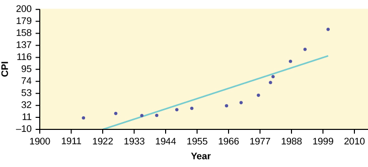
In the example, notice the pattern of the points compared to the line. Although the correlation coefficient is significant, the pattern in the scatterplot indicates that a curve would be a more appropriate model to use than a line. In this example, a statistician should prefer to use other methods to fit a curve to this data, rather than model the data with the line we found. In addition to doing the calculations, it is always important to look at the scatterplot when deciding whether a linear model is appropriate.

If you are interested in seeing more years of data, visit the Bureau of Labor Statistics CPI website ftp://ftp.bls.gov/pub/special.requests/cpi/cpiai.txt; our data is taken from the column entitled "Annual Avg." (third column from the right). For example you could add more current years of data. Try adding the more recent years: 2004: CPI = 188.9; 2008: CPI = 215.3; 2011: CPI = 224.9. See how it affects the model. (Check: ŷ = –4436 + 2.295 x ; r = 0.9018. Is r significant? Is the fit better with the addition of the new points?)

Try it

The following table shows economic development measured in per capita income PCINC.

Year PCINC Year PCINC
1870 340 1920 1050
1880 499 1930 1170
1890 592 1940 1364
1900 757 1950 1836
1910 927 1960 2132
  1. What are the independent and dependent variables?
  2. Draw a scatter plot.
  3. Use regression to find the line of best fit and the correlation coefficient.
  4. Interpret the significance of the correlation coefficient.
  5. Is there a linear relationship between the variables?
  6. Find the coefficient of determination and interpret it.
  7. What is the slope of the regression equation? What does it mean?
  8. Use the line of best fit to estimate PCINC for 1900, for 2000.
  9. Determine if there are any outliers.

a. The independent variable ( x ) is the year and the dependent variable ( y ) is the per capita income.

b.

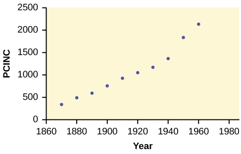
c. ŷ = 18.61x – 34574; r = 0.9732

d. At df = 8, the critical value is 0.632. The r value is significant because it is greater than the critical value.

e. There does appear to be a linear relationship between the variables.

f. The coefficient of determination is 0.947, which means that 94.7% of the variation in PCINC is explained by the variation in the years.

g. and h. The slope of the regression equation is 18.61, and it means that per capita income increases by $18.61 for each passing year. ŷ = 785 when the year is 1900, and ŷ = 2,646 when the year is 2000.

i. There do not appear to be any outliers.

Got questions? Get instant answers now!

95% critical values of the sample correlation coefficient table

Degrees of Freedom: n – 2 Critical Values: (+ and –)
1 0.997
2 0.950
3 0.878
4 0.811
5 0.754
6 0.707
7 0.666
8 0.632
9 0.602
10 0.576
11 0.555
12 0.532
13 0.514
14 0.497
15 0.482
16 0.468
17 0.456
18 0.444
19 0.433
20 0.423
21 0.413
22 0.404
23 0.396
24 0.388
25 0.381
26 0.374
27 0.367
28 0.361
29 0.355
30 0.349
40 0.304
50 0.273
60 0.250
70 0.232
80 0.217
90 0.205
100 0.195

References

Data from the House Ways and Means Committee, the Health and Human Services Department.

Data from Microsoft Bookshelf.

Data from the United States Department of Labor, the Bureau of Labor Statistics.

Data from the Physician’s Handbook, 1990.

Data from the United States Department of Labor, the Bureau of Labor Statistics.

Chapter review

To determine if a point is an outlier, do one of the following:

  1. Input the following equations into the TI 83, 83+,84, 84+:

    y 1 = a + b x y 2 = ( 2 s ) a + b x y 3 = ( 2 s ) a + b x where s is the standard deviation of the residuals

    If any point is above y 2 or below y 3 then the point is considered to be an outlier.

  2. Use the residuals and compare their absolute values to 2 s where s is the standard deviation of the residuals. If the absolute value of any residual is greater than or equal to 2 s , then the corresponding point is an outlier.
  3. Note: The calculator function LinRegTTest (STATS TESTS LinRegTTest) calculates s .

Use the following information to answer the next four exercises. The scatter plot shows the relationship between hours spent studying and exam scores. The line shown is the calculated line of best fit. The correlation coefficient is 0.69.

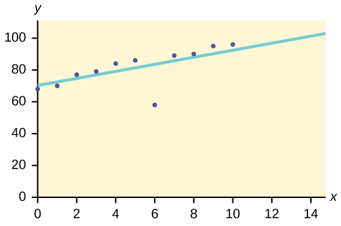
Do there appear to be any outliers?

Yes, there appears to be an outlier at (6, 58).

Got questions? Get instant answers now!

A point is removed, and the line of best fit is recalculated. The new correlation coefficient is 0.98. Does the point appear to have been an outlier? Why?

Got questions? Get instant answers now!

What effect did the potential outlier have on the line of best fit?

The potential outlier flattened the slope of the line of best fit because it was below the data set. It made the line of best fit less accurate is a predictor for the data.

Got questions? Get instant answers now!

Are you more or less confident in the predictive ability of the new line of best fit?

Got questions? Get instant answers now!

The Sum of Squared Errors for a data set of 18 numbers is 49. What is the standard deviation?

s = 1.75

Got questions? Get instant answers now!

The Standard Deviation for the Sum of Squared Errors for a data set is 9.8. What is the cutoff for the vertical distance that a point can be from the line of best fit to be considered an outlier?

Got questions? Get instant answers now!

Questions & Answers

how does Neisseria cause meningitis
Nyibol Reply
what is microbiologist
Muhammad Reply
what is errata
Muhammad
is the branch of biology that deals with the study of microorganisms.
Ntefuni Reply
What is microbiology
Mercy Reply
studies of microbes
Louisiaste
when we takee the specimen which lumbar,spin,
Ziyad Reply
How bacteria create energy to survive?
Muhamad Reply
Bacteria doesn't produce energy they are dependent upon their substrate in case of lack of nutrients they are able to make spores which helps them to sustain in harsh environments
_Adnan
But not all bacteria make spores, l mean Eukaryotic cells have Mitochondria which acts as powerhouse for them, since bacteria don't have it, what is the substitution for it?
Muhamad
they make spores
Louisiaste
what is sporadic nd endemic, epidemic
Aminu Reply
the significance of food webs for disease transmission
Abreham
food webs brings about an infection as an individual depends on number of diseased foods or carriers dully.
Mark
explain assimilatory nitrate reduction
Esinniobiwa Reply
Assimilatory nitrate reduction is a process that occurs in some microorganisms, such as bacteria and archaea, in which nitrate (NO3-) is reduced to nitrite (NO2-), and then further reduced to ammonia (NH3).
Elkana
This process is called assimilatory nitrate reduction because the nitrogen that is produced is incorporated in the cells of microorganisms where it can be used in the synthesis of amino acids and other nitrogen products
Elkana
Examples of thermophilic organisms
Shu Reply
Give Examples of thermophilic organisms
Shu
advantages of normal Flora to the host
Micheal Reply
Prevent foreign microbes to the host
Abubakar
they provide healthier benefits to their hosts
ayesha
They are friends to host only when Host immune system is strong and become enemies when the host immune system is weakened . very bad relationship!
Mark
what is cell
faisal Reply
cell is the smallest unit of life
Fauziya
cell is the smallest unit of life
Akanni
ok
Innocent
cell is the structural and functional unit of life
Hasan
is the fundamental units of Life
Musa
what are emergency diseases
Micheal Reply
There are nothing like emergency disease but there are some common medical emergency which can occur simultaneously like Bleeding,heart attack,Breathing difficulties,severe pain heart stock.Hope you will get my point .Have a nice day ❣️
_Adnan
define infection ,prevention and control
Innocent
I think infection prevention and control is the avoidance of all things we do that gives out break of infections and promotion of health practices that promote life
Lubega
Heyy Lubega hussein where are u from?
_Adnan
en français
Adama
which site have a normal flora
ESTHER Reply
Many sites of the body have it Skin Nasal cavity Oral cavity Gastro intestinal tract
Safaa
skin
Asiina
skin,Oral,Nasal,GIt
Sadik
How can Commensal can Bacteria change into pathogen?
Sadik
How can Commensal Bacteria change into pathogen?
Sadik
all
Tesfaye
by fussion
Asiina
what are the advantages of normal Flora to the host
Micheal
what are the ways of control and prevention of nosocomial infection in the hospital
Micheal
what is inflammation
Shelly Reply
part of a tissue or an organ being wounded or bruised.
Wilfred
what term is used to name and classify microorganisms?
Micheal Reply
Binomial nomenclature
adeolu
Got questions? Join the online conversation and get instant answers!
Jobilize.com Reply

Get Jobilize Job Search Mobile App in your pocket Now!

Get it on Google Play Download on the App Store Now


Source:  OpenStax, Introductory statistics. OpenStax CNX. May 06, 2016 Download for free at http://legacy.cnx.org/content/col11562/1.18
Google Play and the Google Play logo are trademarks of Google Inc.

Notification Switch

Would you like to follow the 'Introductory statistics' conversation and receive update notifications?

Ask