

| << Chapter < Page | Chapter >> Page > |
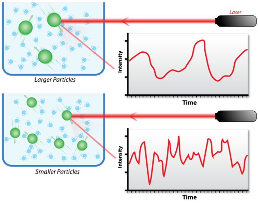
As a result of the Brownian motion, the distance between particles is constantly changing and this results in a Doppler shift between the frequency of the incident light and the frequency of the scattered light. Since the distance between particles also affects the phase overlap/interfering of the diffracted light, the brightness and darkness of the spots in the “speckle” pattern will in turn fluctuate in intensity as a function of time when the particles change position with respect to each other. Then, as the rate of these intensity fluctuations depends on how fast the particles are moving (smaller particles diffuse faster), information about the size distribution of particles in the solution could be acquired by processing the fluctuations of the intensity of scattered light. [link] shows the hypothetical fluctuation of scattering intensity of larger particles and smaller particles.
In order to mathematically process the fluctuation of intensity, there are several principles/terms to be understood. First, the intensity correlation function is used to describe the rate of change in scattering intensity by comparing the intensity I ( t ) at time t to the intensity I ( t + τ ) at a later time ( t + τ), and is quantified and normalized by [link] and [link] , where braces indicate averaging over t .
Second, since it is not possible to know how each particle moves from the fluctuation, the electric field correlation function is instead used to correlate the motion of the particles relative to each other, and is defined by [link] and [link] , where E ( t ) and E ( t + τ ) are the scattered electric fields at times t and t + τ .
For a monodisperse system undergoing Brownian motion, g 1 ( τ ) will decay exponentially with a decay rate Γ which is related by Brownian motion to the diffusivity by [link] , [link] , and [link] , where q is the magnitude of the scattering wave vector and q 2 reflects the distance the particle travels, n is the refraction index of the solution, and θ is angle at which the detector is located.
For a polydisperse system however, g 1 ( τ ) can no longer be represented as a single exponential decay and must be represented as a intensity-weighed integral over a distribution of decay rates G (Γ) by [link] , where G (Γ) is normalized, [link] .
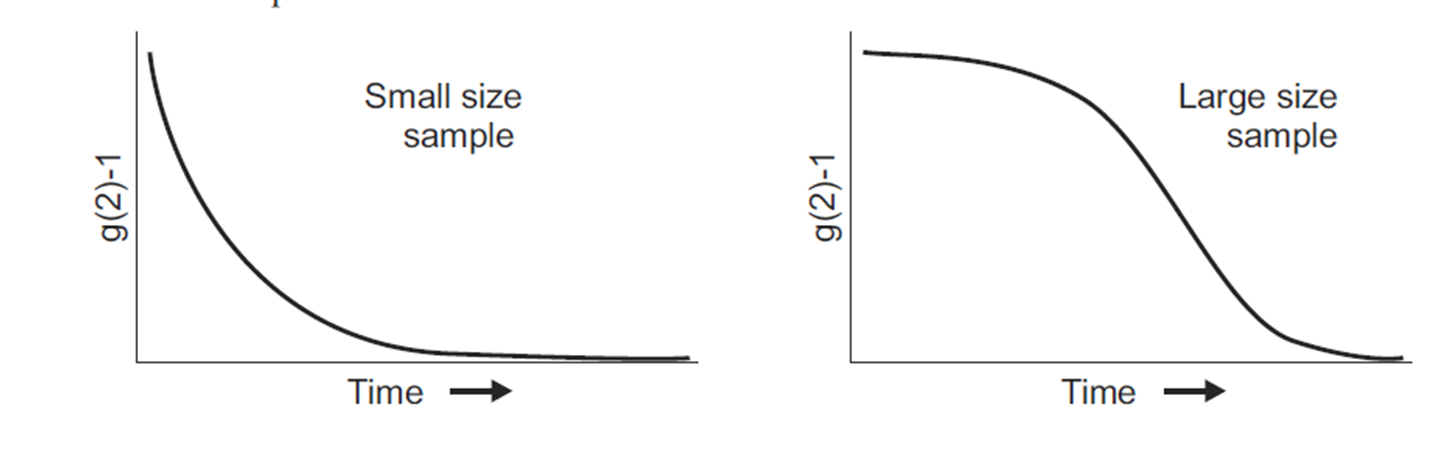
Third, the two correlation functions above can be equated using the Seigert relationship based on the principles of Gaussian random processes (which the scattering light usually is), and can be expressed as [link] , where β is a factor that depends on the experimental geometry, and B is the long-time value of g 2 ( τ ), which is referred to as the baseline and is normally equal to 1. [link] shows the decay of g 2 ( τ ) for small size sample and large size sample.
Notification Switch
Would you like to follow the 'Physical methods in chemistry and nano science' conversation and receive update notifications?

|
|

|
|

|
|

|
|

|
|

|
|
|
|
|

|
|

|
|
|
|