The two types of solutions in the three regions are illustrated in
[link] .
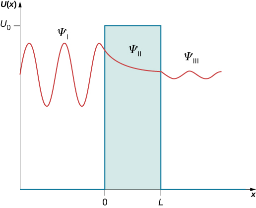
Three types of solutions to the stationary Schrӧdinger equation for the quantum-tunneling problem: Oscillatory behavior in regions I and III where a quantum particle moves freely, and exponential-decay behavior in region II (the barrier region) where the particle moves in the potential
.
Now we use the boundary conditions to find equations for the unknown constants.
[link] and
[link] are substituted into
[link] to give
Similarly, we substitute
[link] and
[link] into
[link] , differentiate, and obtain
Similarly, the boundary condition
[link] reads explicitly
We now have four equations for five unknown constants. However, because the quantity we are after is the transmission coefficient, defined in
[link] by the fraction
F /
A , the number of equations is exactly right because when we divide each of the above equations by
A , we end up having only four unknown fractions:
B /
A ,
C /
A ,
D /
A , and
F /
A , three of which can be eliminated to find
F /
A . The actual algebra that leads to expression for
F /
A is pretty lengthy, but it can be done either by hand or with a help of computer software. The end result is
In deriving
[link] , to avoid the clutter, we use the substitutions
,
We substitute
[link] into
[link] and obtain the exact expression for the transmission coefficient for the barrier,
or
where
For a wide and high barrier that transmits poorly,
[link] can be approximated by
Whether it is the exact expression
[link] or the approximate expression
[link] , we see that the tunneling effect very strongly depends on the width
L of the potential barrier. In the laboratory, we can adjust both the potential height
and the width
L to design nano-devices with desirable transmission coefficients.
Transmission coefficient
Two copper nanowires are insulated by a copper oxide nano-layer that provides a 10.0-eV potential barrier. Estimate the tunneling probability between the nanowires by 7.00-eV electrons through a 5.00-nm thick oxide layer. What if the thickness of the layer were reduced to just 1.00 nm? What if the energy of electrons were increased to 9.00 eV?
Strategy
Treating the insulating oxide layer as a finite-height potential barrier, we use
[link] . We identify
,
,
,
, and
. We use
[link] to compute the exponent. Also, we need the rest mass of the electron
and Planck’s constant
. It is typical for this type of estimate to deal with very small quantities that are often not suitable for handheld calculators. To make correct estimates of orders, we make the conversion
.