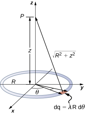
A ring has a uniform charge density
, with units of coulomb per unit meter of arc. Find the electric potential at a point on the axis passing through the center of the ring.
Strategy
We use the same procedure as for the charged wire. The difference here is that the charge is distributed on a circle. We divide the circle into infinitesimal elements shaped as arcs on the circle and use cylindrical coordinates shown in
[link] .
We want to calculate the electric potential due to a ring of charge.
Solution
A general element of the arc between
and
is of length
and therefore contains a charge equal to
The element is at a distance of
from
P , and therefore the potential is
Significance
This result is expected because every element of the ring is at the same distance from point
P . The net potential at
P is that of the total charge placed at the common distance,
.
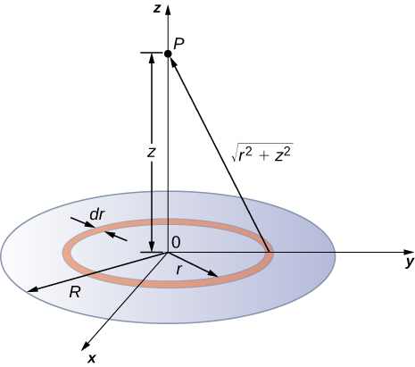
A disk of radius
R has a uniform charge density
, with units of coulomb meter squared. Find the electric potential at any point on the axis passing through the center of the disk.
Strategy
We divide the disk into ring-shaped cells, and make use of the result for a ring worked out in the previous example, then integrate over
r in addition to
. This is shown in
[link] .
We want to calculate the electric potential due to a disk of charge.
Solution
An infinitesimal width cell between cylindrical coordinates
r and
shown in
[link] will be a ring of charges whose electric potential
at the field point has the following expression
where
The superposition of potential of all the infinitesimal rings that make up the disk gives the net potential at point
P . This is accomplished by integrating from
to
:
Significance
The basic procedure for a disk is to first integrate around
and then over
r . This has been demonstrated for uniform (constant) charge density. Often, the charge density will vary with
r , and then the last integral will give different results.
Find the electric potential due to an infinitely long uniformly charged wire.
Strategy
Since we have already worked out the potential of a finite wire of length
L in
[link] , we might wonder if taking
in our previous result will work:
However, this limit does not exist because the argument of the logarithm becomes [2/0] as
, so this way of finding
V of an infinite wire does not work. The reason for this problem may be traced to the fact that the charges are not localized in some space but continue to infinity in the direction of the wire. Hence, our (unspoken) assumption that zero potential must be an infinite distance from the wire is no longer valid.
To avoid this difficulty in calculating limits, let us use the definition of potential by integrating over the electric field from the previous section, and the value of the electric field from this charge configuration from the previous chapter.
Solution
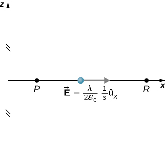
We use the integral
where
R is a finite distance from the line of charge, as shown in
[link] .
Points of interest for calculating the potential of an infinite line of charge.
With this setup, we use
and
to obtain
Now, if we define the reference potential
at
this simplifies to
Note that this form of the potential is quite usable; it is 0 at 1 m and is undefined at infinity, which is why we could not use the latter as a reference.
Significance
Although calculating potential directly can be quite convenient, we just found a system for which this strategy does not work well. In such cases, going back to the definition of potential in terms of the electric field may offer a way forward.