

| << Chapter < Page | Chapter >> Page > |
The reason is that the sources of the electric field are outside the box. Therefore, if any electric field line enters the volume of the box, it must also exit somewhere on the surface because there is no charge inside for the lines to land on. Therefore, quite generally, electric flux through a closed surface is zero if there are no sources of electric field, whether positive or negative charges, inside the enclosed volume. In general, when field lines leave (or “flow out of”) a closed surface, is positive; when they enter (or “flow into”) the surface, is negative.
Any smooth, non-flat surface can be replaced by a collection of tiny, approximately flat surfaces, as shown in [link] . If we divide a surface S into small patches, then we notice that, as the patches become smaller, they can be approximated by flat surfaces. This is similar to the way we treat the surface of Earth as locally flat, even though we know that globally, it is approximately spherical.
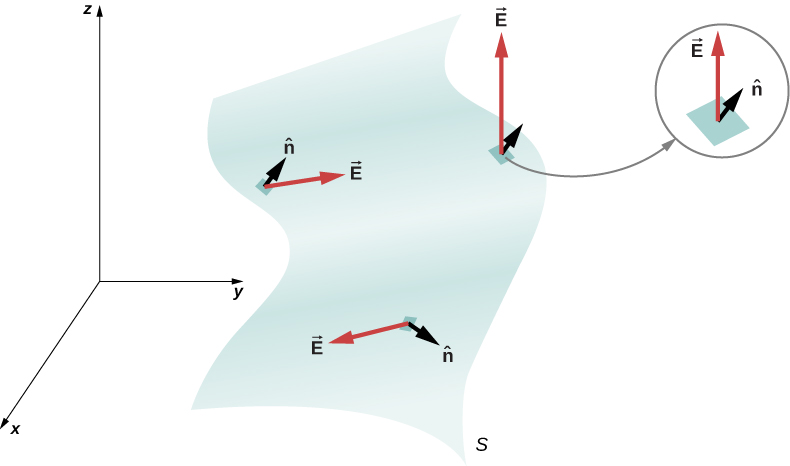
To keep track of the patches, we can number them from 1 through N . Now, we define the area vector for each patch as the area of the patch pointed in the direction of the normal. Let us denote the area vector for the i th patch by (We have used the symbol to remind us that the area is of an arbitrarily small patch.) With sufficiently small patches, we may approximate the electric field over any given patch as uniform. Let us denote the average electric field at the location of the i th patch by
Therefore, we can write the electric flux through the area of the i th patch as
The flux through each of the individual patches can be constructed in this manner and then added to give us an estimate of the net flux through the entire surface S , which we denote simply as .
This estimate of the flux gets better as we decrease the size of the patches. However, when you use smaller patches, you need more of them to cover the same surface. In the limit of infinitesimally small patches, they may be considered to have area dA and unit normal . Since the elements are infinitesimal, they may be assumed to be planar, and may be taken as constant over any element. Then the flux through an area dA is given by It is positive when the angle between and is less than and negative when the angle is greater than . The net flux is the sum of the infinitesimal flux elements over the entire surface. With infinitesimally small patches, you need infinitely many patches, and the limit of the sum becomes a surface integral. With representing the integral over S ,
In practical terms, surface integrals are computed by taking the antiderivatives of both dimensions defining the area, with the edges of the surface in question being the bounds of the integral.
To distinguish between the flux through an open surface like that of [link] and the flux through a closed surface (one that completely bounds some volume), we represent flux through a closed surface by
Notification Switch
Would you like to follow the 'University physics volume 2' conversation and receive update notifications?

|
|

|
|

|
|

|
|

|
|

|
|

|
|

|
|

|
|
|
|