

| << Chapter < Page | Chapter >> Page > |
Now that we have some experience calculating electric fields, let’s try to gain some insight into the geometry of electric fields. As mentioned earlier, our model is that the charge on an object (the source charge) alters space in the region around it in such a way that when another charged object (the test charge) is placed in that region of space, that test charge experiences an electric force. The concept of electric field line s , and of electric field line diagrams, enables us to visualize the way in which the space is altered, allowing us to visualize the field. The purpose of this section is to enable you to create sketches of this geometry, so we will list the specific steps and rules involved in creating an accurate and useful sketch of an electric field.
It is important to remember that electric fields are three-dimensional. Although in this book we include some pseudo-three-dimensional images, several of the diagrams that you’ll see (both here, and in subsequent chapters) will be two-dimensional projections, or cross-sections. Always keep in mind that in fact, you’re looking at a three-dimensional phenomenon.
Our starting point is the physical fact that the electric field of the source charge causes a test charge in that field to experience a force. By definition, electric field vectors point in the same direction as the electric force that a (hypothetical) positive test charge would experience, if placed in the field ( [link] )
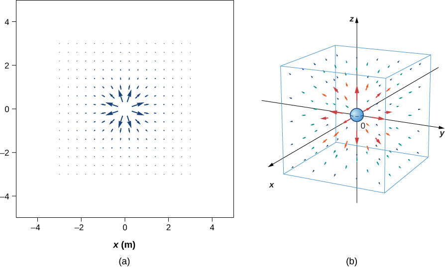
We’ve plotted many field vectors in the figure, which are distributed uniformly around the source charge. Since the electric field is a vector, the arrows that we draw correspond at every point in space to both the magnitude and the direction of the field at that point. As always, the length of the arrow that we draw corresponds to the magnitude of the field vector at that point. For a point source charge, the length decreases by the square of the distance from the source charge. In addition, the direction of the field vector is radially away from the source charge, because the direction of the electric field is defined by the direction of the force that a positive test charge would experience in that field. (Again, keep in mind that the actual field is three-dimensional; there are also field lines pointing out of and into the page.)
This diagram is correct, but it becomes less useful as the source charge distribution becomes more complicated. For example, consider the vector field diagram of a dipole ( [link] ).
Notification Switch
Would you like to follow the 'University physics volume 2' conversation and receive update notifications?

|
|

|
|

|
|

|
|

|
|

|
|

|
|

|
|

|
|

|