

| << Chapter < Page | Chapter >> Page > |
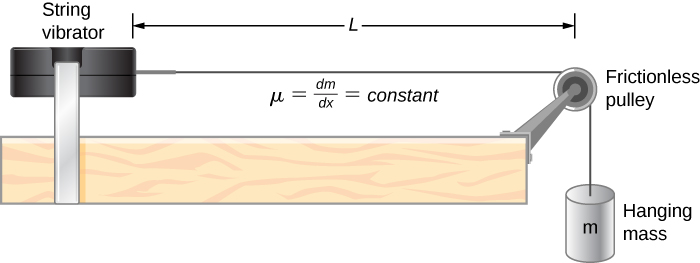
The lab setup shows a string attached to a string vibrator, which oscillates the string with an adjustable frequency f . The other end of the string passes over a frictionless pulley and is tied to a hanging mass. The magnitude of the tension in the string is equal to the weight of the hanging mass. The string has a constant linear density (mass per length) and the speed at which a wave travels down the string equals [link] . The symmetrical boundary conditions (a node at each end) dictate the possible frequencies that can excite standing waves. Starting from a frequency of zero and slowly increasing the frequency, the first mode appears as shown in [link] . The first mode, also called the fundamental mode or the first harmonic, shows half of a wavelength has formed, so the wavelength is equal to twice the length between the nodes . The fundamental frequency , or first harmonic frequency, that drives this mode is
where the speed of the wave is Keeping the tension constant and increasing the frequency leads to the second harmonic or the mode. This mode is a full wavelength and the frequency is twice the fundamental frequency:
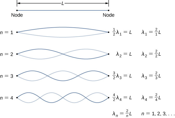
The next two modes, or the third and fourth harmonics, have wavelengths of and driven by frequencies of and All frequencies above the frequency are known as the overtone s . The equations for the wavelength and the frequency can be summarized as:
The standing wave patterns that are possible for a string, the first four of which are shown in [link] , are known as the normal mode s , with frequencies known as the normal frequencies. In summary, the first frequency to produce a normal mode is called the fundamental frequency (or first harmonic). Any frequencies above the fundamental frequency are overtones. The second frequency of the normal mode of the string is the first overtone (or second harmonic). The frequency of the normal mode is the second overtone (or third harmonic) and so on.
The solutions shown as [link] and [link] are for a string with the boundary condition of a node on each end. When the boundary condition on either side is the same, the system is said to have symmetric boundary conditions. [link] and [link] are good for any symmetric boundary conditions, that is, nodes at both ends or antinodes at both ends.
Notification Switch
Would you like to follow the 'University physics volume 1' conversation and receive update notifications?

|
|

|
|

|
|

|
|

|
|

|
|

|
|

|
|
|
|
|

|