

| << Chapter < Page | Chapter >> Page > |
This chapter gives you an opportunity to build on what you have learned in previous grades about data handling and probability. The work done will be mostly of a practical nature. Through problem solving and activities, you will end up mastering further methods of collecting, organising, displaying and analysing data. You will also learn how to interpret data, and not always to accept the data at face value, because data is sometimes misused and abused in order to try to falsely prove or support a viewpoint. Measures of central tendency (mean, median and mode) and dispersion (range, percentiles, quartiles, inter-quartile, semi-inter-quartile range, variance and standard deviation) will be investigated. Of course, the activities involving probability will be familiar to most of you - for example, you may have played dice or card games even before you came to school. Your basic understanding of probability and chance gained so far will be deepened to enable you to come to a better understanding of how chance and uncertainty can be measured and understood.
The measures of central tendency (mean, median and mode) and measures of dispersion (quartiles, percentiles, ranges) provide information on the data values at the centre of the data set and provide information on the spread of the data. The information on the spread of the data is however based on data values at specific points in the data set, e.g. the end points for range and data points that divide the data set into 4 equal groups for the quartiles. The behaviour of the entire data set is therefore not examined.
A method of determining the spread of data is by calculating a measure of the possible distances between the data and the mean. The two important measures that are used are called the variance and the standard deviation of the data set.
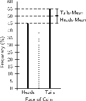
The variance of a data set is the average squared distance between the mean of the data set and each data value. An example of what this means is shown in [link] . The graph represents the results of 100 tosses of a fair coin, which resulted in 45 heads and 55 tails. The mean of the results is 50. The squared distance between the heads value and the mean is and the squared distance between the tails value and the mean is . The average of these two squared distances gives the variance, which is .
Let the population consist of elements , with mean (read as "x bar"). The variance of the population, denoted by , is the average of the square of the distance of each data value from the mean value.
Since the population variance is squared, it is not directly comparable with the mean and the data themselves.
Let the sample consist of the elements , taken from the population, with mean . The variance of the sample, denoted by , is the average of the squared deviations from the sample mean:
Since the sample variance is squared, it is also not directly comparable with the mean and the data themselves.
Notification Switch
Would you like to follow the 'Siyavula textbooks: grade 11 maths' conversation and receive update notifications?

|
|

|
|

|
|

|
|

|
|

|
|

|
|
|
|
|

|
|

|