Signal recovery via ℓ_1 minimization

As we will see later in this course , there now exist a wide variety of approaches to recover a sparse signal $x$ from a small number of linear measurements. We begin by considering a natural first approach to the problem of sparse recovery.

Given measurements $y=\Phi x$ and the knowledge that our original signal $x$ is sparse or compressible , it is natural to attempt to recover $x$ by solving an optimization problem of the form

where $\mathcal{B}\left(y\right)$ ensures that $\widehat{x}$ is consistent with the measurements $y$ . Recall that ${∥z∥}_0=\left|\mathrm{supp}\left(z\right)\right|$ simply counts the number of nonzero entries in $z$ , so [link] simply seeks out the sparsest signal consistent with the observed measurements. For example, if our measurements are exact and noise-free, then we can set $\mathcal{B}\left(y\right)=\{z:\Phi z=y\}$ . When the measurements have been contaminated with a small amount of bounded noise, we could instead set $\mathcal{B}\left(y\right)=\{z:{∥\Phi ,z,-,y∥}_2\le ϵ\}$ . In both cases, [link] finds the sparsest $x$ that is consistent with the measurements $y$ .

Note that in [link] we are inherently assuming that $x$ itself is sparse. In the more common setting where $x=\Psi \alpha$ , we can easily modify the approach and instead consider

where $\mathcal{B}\left(y\right)=\{z:\Phi \Psi z=y\}$ or $\mathcal{B}\left(y\right)=\{z:{∥\Phi ,\Psi ,z,-,y∥}_2\le ϵ\}$ . By setting $\tilde{\Phi }=\Phi \Psi$ we see that [link] and [link] are essentially identical. Moreover, as noted in "Matrices that satisfy the RIP" , in many cases the introduction of $\Psi$ does not significantly complicate the construction of matrices $\Phi$ such that $\tilde{\Phi }$ will satisfy the desired properties. Thus, for most of the remainder of this course we will restrict our attention to the case where $\Psi =I$ . It is important to note, however, that this restriction does impose certain limits in our analysis when $\Psi$ is a general dictionary and not an orthonormal basis. For example, in this case ${∥\widehat{x},-,x∥}_2={∥\Psi ,\widehat{c},-,\Psi ,c∥}_2\ne {∥\widehat{\alpha },-,\alpha ∥}_2$ , and thus a bound on ${∥\widehat{c},-,c∥}_2$ cannot directly be translated into a bound on $∥\widehat{x},-,x∥$ , which is often the metric of interest.

Although it is possible to analyze the performance of [link] under the appropriate assumptions on $\Phi$ , we do not pursue this strategy since the objective function ${∥·∥}_0$ is nonconvex, and hence [link] is potentially very difficult to solve. In fact, one can show that for a general matrix $\Phi$ , even finding a solution that approximates the true minimum is NP-hard. One avenue for translating this problem into something more tractable is to replace ${∥·∥}_0$ with its convex approximation ${∥·∥}_1$ . Specifically, we consider

Provided that $\mathcal{B}\left(y\right)$ is convex, [link] is computationally feasible. In fact, when $\mathcal{B}\left(y\right)=\{z:\Phi z=y\}$ , the resulting problem can be posed as a linear program  [link] .

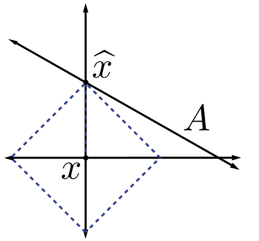
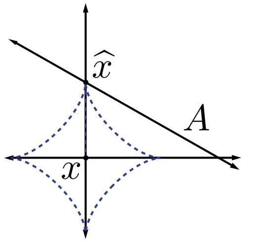
It is clear that replacing [link] with [link] transforms a computationally intractable problem into a tractable one, but it may not be immediately obvious that the solution to [link] will be at all similar to the solution to [link] . However, there are certainly intuitive reasons to expect that the use of ${\ell }_1$ minimization will indeed promote sparsity. As an example, recall the example we discussed earlier shown in [link] . In this case the solutions to the ${\ell }_1$ minimization problem coincided exactly with the solution to the ${\ell }_p$ minimization problem for any $p<1$ , and notably, is sparse. Moreover, the use of ${\ell }_1$ minimization to promote or exploit sparsity has a long history, dating back at least to the work of Beurling on Fourier transform extrapolation from partial observations  [link] .

Additionally, in a somewhat different context, in 1965 Logan  [link] showed that a bandlimited signal can be perfectly recovered in the presence of arbitrary corruptions on a small interval. Again, the recovery method consists of searching for the bandlimited signal that is closest to the observed signal in the ${\ell }_1$ norm. This can be viewed as further validation of the intuition gained from [link] — the ${\ell }_1$ norm is well-suited to sparse errors.

Historically, the use of ${\ell }_1$ minimization on large problems finally became practical with the explosion of computing power in the late 1970's and early 1980's. In one of its first applications, it was demonstrated that geophysical signals consisting of spike trains could be recovered from only the high-frequency components of these signals by exploiting ${\ell }_1$ minimization  [link] , [link] , [link] . Finally, in the 1990's there was renewed interest in these approaches within the signal processing community for the purpose of finding sparse approximations to signals and images when represented in overcomplete dictionaries or unions of bases  [link] , [link] . Separately, ${\ell }_1$ minimization received significant attention in the statistics literature as a method for variable selection in linear regression , known as the Lasso  [link] .

Thus, there are a variety of reasons to suspect that ${\ell }_1$ minimization will provide an accurate method for sparse signal recovery. More importantly, this also provides a computationally tractable approach to the sparse signal recovery problem. We now provide an overview of ${\ell }_1$ minimization in both the noise-free and noisy settings from a theoretical perspective. We will then further discuss algorithms for performing ${\ell }_1$ minimization later in this course .