Fir digital filters  (Page 2/7)

Frequency-domain description of fir filters

The output of a length-N FIR filter can be calculated from the input using convolution.

and the transfer function of an FIR filter is given by the z-transform of the finite length impulse response $h\left(n\right)$ as

The frequency response of a filter, is found by setting $z=e^{j\omega }$ , which is the same as the discrete-time Fourier transform (DTFT) of $h\left(n\right)$ , which gives

with $\omega$ being frequency in radians per second. Strictly speaking, the exponent should be $-j\omega Tn$ where $T$ is the time interval between the integer steps of $n$ (the sampling interval). But to simplify notation, it will be assumed that $T=1$ until later in the notes where the relation between $n$ and time is more important. Also to simplify notation, $H\left(\omega \right)$ is used to represent the frequency response rather that $H\left(e^{j\omega }\right)$ . It should always be clear from the context whether $H$ is a function of $z$ or $\omega$ .

This frequency-response function is complex-valued and consists of a magnitude and a phase. Even though the impulseresponse is a function of the discrete variable $n$ , the frequency response is a function of the continuous-frequencyvariable $\omega$ and is periodic with period $2\pi$ . This periodicity is easily shown by

with frequency denoted by $\omega$ in radians per second or by $f$ in Hz (hertz or cycles per second). These are related by

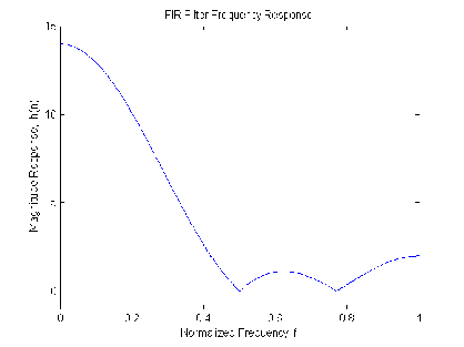
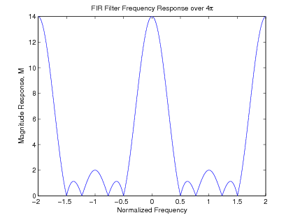
An example of a length-5 filter might be

with a frequency-response plot shown over the base frequency band ( $0<\omega <\pi$ or $0<f<1$ in [link] . To illustrate the periodic nature of the total frequency response, [link] shows the response over a wider set of frequencies.

The Discrete Fourier Transform (DFT) can be used to evaluate the frequency response at certain frequencies. The DFT [link] of the length-N impulse response $h\left(n\right)$ is defined as

which, when compared to [link] , gives

for ${\omega }_k=2\pi k/N$ .

This states that the DFT of $h\left(n\right)$ gives $N$ samples of the frequency-response function $H\left(\omega \right)$ . This sampling at $N$ points may not give enough detail, and, therefore, more samples areneeded. Any number of equally spaced samples can be found with the DFT by simply appending $L-N$ zeros to $h\left(n\right)$ and taking an L-length DFT. This is often useful when an accurate picture ofall of $H\left(\omega \right)$ is required. Indeed, when the number of appended zeros goes to infinity, the DFT becomes the discrete-time Fourier transform of $h\left(n\right)$ .

The fact that the DFT of $h\left(n\right)$ is a set of $N$ samples of the frequency response suggests a method of designing FIR filters inwhich the inverse DFT of $N$ samples of a desired frequency response gives the filter coefficients $h\left(n\right)$ . That approach is called frequency sampling and is developed in another section.

Linear-phase fir filters

A particular property of FIR filters that has proven to be very powerful is that a linear phase shift for the frequency response is possible. Thisis especially important to time domain details of a signal. The spectrum of a signal contains the individual frequency domain components separatedin frequency. The process of filtering usually involves passing some of these components and rejecting others. This is done by multiplying thedesired ones by one and the undesired ones by zero. When they are recombined, it is important that the components have the same time domainalignment as they originally did. That is exactly what linear phase insures. A phase response that is linear with frequency keeps all of thefrequency components properly registered with each other. That is especially important in seismic, radar, and sonar signal analysis as wellas for many medical signals where the relative time locations of events contains the information of interest.