<< Chapter < Page Chapter >> Page >
Continuous Random Variables: Introduction is part of the collection col10555 written by Barbara Illowsky and Susan Dean and serves as an introduction to the uniform and exponential distributions with contributions from Roberta Bloom.

Student learning outcomes

By the end of this chapter, the student should be able to:

  • Recognize and understand continuous probability density functions in general.
  • Recognize the uniform probability distribution and apply it appropriately.
  • Recognize the exponential probability distribution and apply it appropriately.

Introduction

Continuous random variables have many applications. Baseball batting averages, IQ scores, the length of time a long distance telephone call lasts, the amount of money a person carries, thelength of time a computer chip lasts, and SAT scores are just a few. The field of reliability depends on a variety of continuous random variables.

This chapter gives an introduction to continuous random variables and the many continuous distributions. We will be studying these continuous distributions for several chapters.

The values of discrete and continuous random variables can be ambiguous. For example, if X is equal to the number of miles (to the nearest mile) you drive to work, then X is a discrete random variable. You count the miles. If X is the distance you drive to work, then you measure values of X and X is a continuous random variable. How the random variable is defined is very important.

Properties of continuous probability distributions

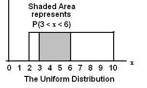
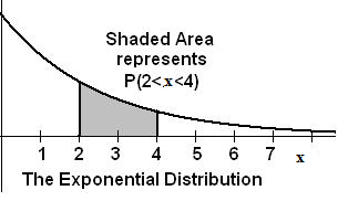
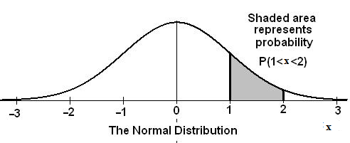
The graph of a continuous probability distribution is a curve. Probability is represented by area under the curve.

The curve is called the probability density function (abbreviated: pdf ). We use the symbol f x to represent the curve. f x is the function that corresponds to the graph; we use the density function f x to draw the graph of the probability distribution.

Area under the curve is given by a different function called the cumulative distribution function (abbreviated: cdf ). The cumulative distribution function is used to evaluate probability as area.

  • The outcomes are measured, not counted.
  • The entire area under the curve and above the x-axis is equal to 1.
  • Probability is found for intervals of x values rather than for individual x values.
  • P ( c x d ) is the probability that the random variable X is in the interval between the values c and d. P ( c x d ) is the area under the curve, above the x-axis, to the right of c and the left of d.
  • P ( x c ) 0 The probability that x takes on any single individual value is 0. The area below the curve, above the x-axis, and between x=c and x=c has no width, and therefore no area (area = 0). Since the probability is equal to the area, the probability is also 0.

We will find the area that represents probability by using geometry, formulas, technology, or probability tables. In general, calculus is needed to find the area under the curve for many probability density functions. When we use formulas to find the area in this textbook, the formulas were found by using the techniques of integral calculus. However, because most students taking this course have not studied calculus, we will not be using calculus in this textbook.

There are many continuous probability distributions. When using a continuous probability distribution to model probability, the distribution used is selected to best model and fit the particular situation.

In this chapter and the next chapter, we will study the uniform distribution, the exponential distribution, and the normal distribution. The following graphs illustrate these distributions.

The graph shows a Uniform Distribution with the area between x=3 and x=6 shaded to represent the probability that the value of the random variable X is in the interval between 3 and 6.
The graph shows an Exponential Distribution with the area between x=2 and x=4 shaded to represent the probability that the value of the random variable X is in the interval between 2 and 4.
The graph shows the Standard Normal Distribution with the area between x=1 and x=2 shaded to represent the probability that the value of the random variable X is in the interval between 1 and 2.

**With contributions from Roberta Bloom

Questions & Answers

Ayele, K., 2003. Introductory Economics, 3rd ed., Addis Ababa.
Widad Reply
can you send the book attached ?
Ariel
?
Ariel
What is economics
Widad Reply
the study of how humans make choices under conditions of scarcity
AI-Robot
U(x,y) = (x×y)1/2 find mu of x for y
Desalegn Reply
U(x,y) = (x×y)1/2 find mu of x for y
Desalegn
what is ecnomics
Jan Reply
this is the study of how the society manages it's scarce resources
Belonwu
what is macroeconomic
John Reply
macroeconomic is the branch of economics which studies actions, scale, activities and behaviour of the aggregate economy as a whole.
husaini
etc
husaini
difference between firm and industry
husaini Reply
what's the difference between a firm and an industry
Abdul
firm is the unit which transform inputs to output where as industry contain combination of firms with similar production 😅😅
Abdulraufu
Suppose the demand function that a firm faces shifted from Qd  120 3P to Qd  90  3P and the supply function has shifted from QS  20  2P to QS 10  2P . a) Find the effect of this change on price and quantity. b) Which of the changes in demand and supply is higher?
Toofiq Reply
explain standard reason why economic is a science
innocent Reply
factors influencing supply
Petrus Reply
what is economic.
Milan Reply
scares means__________________ends resources. unlimited
Jan
economics is a science that studies human behaviour as a relationship b/w ends and scares means which have alternative uses
Jan
calculate the profit maximizing for demand and supply
Zarshad Reply
Why qualify 28 supplies
Milan
what are explicit costs
Nomsa Reply
out-of-pocket costs for a firm, for example, payments for wages and salaries, rent, or materials
AI-Robot
concepts of supply in microeconomics
David Reply
economic overview notes
Amahle Reply
identify a demand and a supply curve
Salome Reply
i don't know
Parul
there's a difference
Aryan
Demand curve shows that how supply and others conditions affect on demand of a particular thing and what percent demand increase whith increase of supply of goods
Israr
Hi Sir please how do u calculate Cross elastic demand and income elastic demand?
Abari
Got questions? Join the online conversation and get instant answers!
Jobilize.com Reply
Practice Key Terms 2

Get Jobilize Job Search Mobile App in your pocket Now!

Get it on Google Play Download on the App Store Now


Source:  OpenStax, Collaborative statistics. OpenStax CNX. Jul 03, 2012 Download for free at http://cnx.org/content/col10522/1.40
Google Play and the Google Play logo are trademarks of Google Inc.

Notification Switch

Would you like to follow the 'Collaborative statistics' conversation and receive update notifications?

Ask