

| << Chapter < Page | Chapter >> Page > |
So far in the book, we’ve covered the tough things you need to know to do parallel processing. At this point, assuming that your loops are clean, they use unit stride, and the iterations can all be done in parallel, all you have to do is turn on a compiler flag and buy a good parallel processor. For example, look at the following code:
PARAMETER(NITER=300,N=1000000)
      REAL*8 A(N),X(N),B(N),CDO ITIME=1,NITER
        DO I=1,NA(I) = X(I) + B(I) * C
        ENDDOCALL WHATEVER(A,X,B,C)
      ENDDO
Here we have an iterative code that satisfies all the criteria for a good parallel loop. On a good parallel processor with a modern compiler, you are two flags away from executing in parallel. On Sun Solaris systems, the
autopar flag turns on the automatic parallelization, and the
loopinfo flag causes the compiler to describe the particular optimization performed for each loop. To compile this code under Solaris, you simply add these flags to your
f77 call:
E6000: f77 -O3 -autopar -loopinfo -o daxpy daxpy.f
      daxpy.f:"daxpy.f", line 6: not parallelized, call may be unsafe
      "daxpy.f", line 8: PARALLELIZEDE6000: /bin/time daxpyreal       30.9
      user       30.7sys         0.1
      E6000:
If you simply run the code, it’s executed using one thread. However, the code is enabled for parallel processing for those loops that can be executed in parallel. To execute the code in parallel, you need to set the UNIX environment to the number of parallel threads you wish to use to execute the code. On Solaris, this is done using the
PARALLEL variable:
E6000: setenv PARALLEL 1
      E6000: /bin/time daxpyreal        30.9user        30.7
      sys          0.1E6000: setenv PARALLEL 2
      E6000: /bin/time daxpyreal        15.6
      user        31.0sys          0.2
      E6000: setenv PARALLEL 4E6000: /bin/time daxpyreal        8.2
      user       32.0sys         0.5
      E6000: setenv PARALLEL 8E6000: /bin/time daxpy

      real        4.3user       33.0
      sys         0.8
Speedup is the term used to capture how much faster the job runs using N processors compared to the performance on one processor. It is computed by dividing the single processor time by the multiprocessor time for each number of processors. [link] shows the wall time and speedup for this application.
Improving performance by adding processors
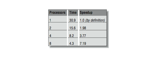
[link] shows this information graphically, plotting speedup versus the number of processors.
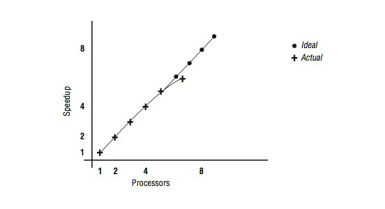
Note that for a while we get nearly perfect speedup, but we begin to see a measurable drop in speedup at four and eight processors. There are several causes for this. In all parallel applications, there is some portion of the code that can’t run in parallel. During those nonparallel times, the other processors are waiting for work and aren’t contributing to efficiency. This nonparallel code begins to affect the overall performance as more processors are added to the application.
So you say, “this is more like it!” and immediately try to run with 12 and 16 threads. Now, we see the graph in [link] and the data from [link] .
Notification Switch
Would you like to follow the 'High performance computing' conversation and receive update notifications?

|
|

|
|

|
|

|
|

|
|

|
|

|
|

|
|
|
|
|

|