

| << Chapter < Page | Chapter >> Page > |
Exponential growth is possible only when infinite natural resources are available; this is not the case in the real world. Charles Darwin recognized this fact in his description of the “struggle for existence,” which states that individuals will compete (with members of their own or other species) for limited resources. The successful ones will survive to pass on their own characteristics and traits (which we know now are transferred by genes) to the next generation at a greater rate (natural selection). To model the reality of limited resources, population ecologists developed the logistic growth model.
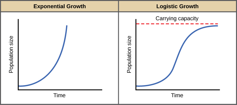
In the real world, with its limited resources, exponential growth cannot continue indefinitely. Exponential growth may occur in environments where there are few individuals and plentiful resources, but when the number of individuals gets large enough, resources will be depleted, slowing the growth rate. Eventually, the growth rate will plateau or level off ( [link] ). This population size, which represents the maximum population size that a particular environment can support, is called the carrying capacity, or K .
The formula we use to calculate logistic growth adds the carrying capacity as a moderating force in the growth rate. The expression “ K – N ” is indicative of how many individuals may be added to a population at a given stage, and “ K – N ” divided by “ K ” is the fraction of the carrying capacity available for further growth. Thus, the exponential growth model is restricted by this factor to generate the logistic growth equation:
Notice that when N is very small, ( K-N )/ K becomes close to K/K or 1, and the right side of the equation reduces to r max N , which means the population is growing exponentially and is not influenced by carrying capacity. On the other hand, when N is large, ( K-N )/ K come close to zero, which means that population growth will be slowed greatly or even stopped. Thus, population growth is greatly slowed in large populations by the carrying capacity K . This model also allows for the population of a negative population growth, or a population decline. This occurs when the number of individuals in the population exceeds the carrying capacity (because the value of (K-N)/K is negative).
A graph of this equation yields an S-shaped curve ( [link] ), and it is a more realistic model of population growth than exponential growth. There are three different sections to an S-shaped curve. Initially, growth is exponential because there are few individuals and ample resources available. Then, as resources begin to become limited, the growth rate decreases. Finally, growth levels off at the carrying capacity of the environment, with little change in population size over time.
Notification Switch
Would you like to follow the 'Principles of biology' conversation and receive update notifications?

|
|

|
|

|
|

|
|

|
|

|
|

|
|

|
|

|
|

|