

| << Chapter < Page | Chapter >> Page > |
The concept of an indifference curve applies to tradeoffs in any household choice, including the labor-leisure choice or the intertemporal choice between present and future consumption. In the labor-leisure choice, each indifference curve shows the combinations of leisure and income that provide a certain level of utility. In an intertemporal choice, each indifference curve shows the combinations of present and future consumption that provide a certain level of utility. The general shapes of the indifference curves—downward sloping, steeper on the left and flatter on the right—also remain the same.
A Labor-Leisure Example
Petunia is working at a job that pays $12 per hour but she gets a raise to $20 per hour. After family responsibilities and sleep, she has 80 hours per week available for work or leisure. As shown in [link] , the highest level of utility for Petunia, on her original budget constraint, is at choice A, where it is tangent to the lower indifference curve (Ul). Point A has 30 hours of leisure and thus 50 hours per week of work, with income of $600 per week (that is, 50 hours of work at $12 per hour). Petunia then gets a raise to $20 per hour, which shifts her budget constraint to the right. Her new utility-maximizing choice occurs where the new budget constraint is tangent to the higher indifference curve Uh. At B, Petunia has 40 hours of leisure per week and works 40 hours, with income of $800 per week (that is, 40 hours of work at $20 per hour).
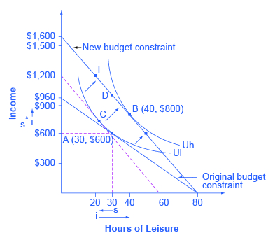
Substitution and income effects provide a vocabulary for discussing how Petunia reacts to a higher hourly wage. The dashed line serves as the tool for separating the two effects on the graph.
The substitution effect tells how Petunia would have changed her hours of work if her wage had risen, so that income was relatively cheaper to earn and leisure was relatively more expensive, but if she had remained at the same level of utility. The slope of the budget constraint in a labor-leisure diagram is determined by the wage rate. Thus, the dashed line is carefully inserted with the slope of the new opportunity set, reflecting the labor-leisure tradeoff of the new wage rate, but tangent to the original indifference curve, showing the same level of utility or “buying power.” The shift from original choice A to point C, which is the point of tangency between the original indifference curve and the dashed line, shows that because of the higher wage, Petunia will want to consume less leisure and more income. The “s” arrows on the horizontal and vertical axes of [link] show the substitution effect on leisure and on income.
Notification Switch
Would you like to follow the 'Openstax microeconomics in ten weeks' conversation and receive update notifications?

|
|

|
|

|
|

|
|

|
|

|
|

|
|

|
|

|
|

|