7.2 Using the central limit theorem

Examples of the central limit theorem

Law of large numbers

The law of large numbers says that if you take samples of larger and larger size from any population, then the mean of the sampling distribution, ${\mu }_{\bar{x}}$ tends to get closer and closer to the true population mean, μ . From the Central Limit Theorem, we know that as n gets larger and larger, the sample means follow a normal distribution. The larger n gets, the smaller the standard deviation of the sampling distribution gets. (Remember that the standard deviation for the sampling distribution of $\bar{X}$ is $\frac{\sigma }{\sqrt{n}}$ .) This means that the sample mean $\bar{x}$ must be closer to the population mean μ as n increases. We can say that μ is the value that the sample means approach as n gets larger. The Central Limit Theorem illustrates the law of large numbers.

This concept is so important and plays such a critical role in what follows it deserves to be developed further. Indeed, there are two critical issues that flow from the Central Limit Theorem and the application of the Law of Large numbers to it. These are

1. The probability density function of the sampling distribution of means is normally distributed regardless of the underlying distribution of the population observations and
2. standard deviation of the sampling distribution decreases as the size of the samples that were used to calculate the means for the sampling distribution increases.

Taking these in order. It would seem counterintuitive that the population may have any distribution and the distribution of means coming from it would be normally distributed. With the use of computers, experiments can be simulated that show the process by which the sampling distribution changes as the sample size is increased. These simulations show visually the results of the mathematical proof of the Central Limit Theorem.

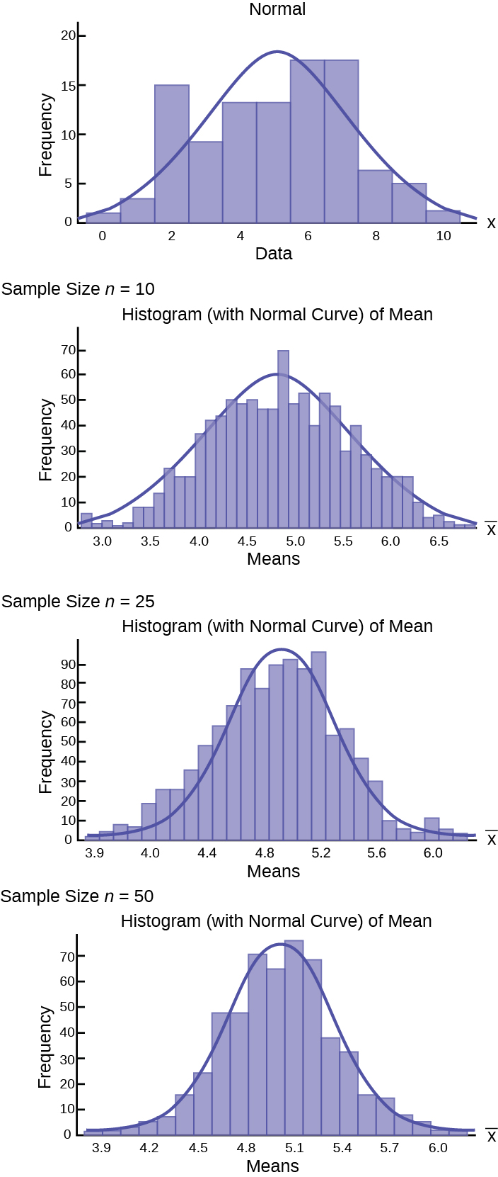
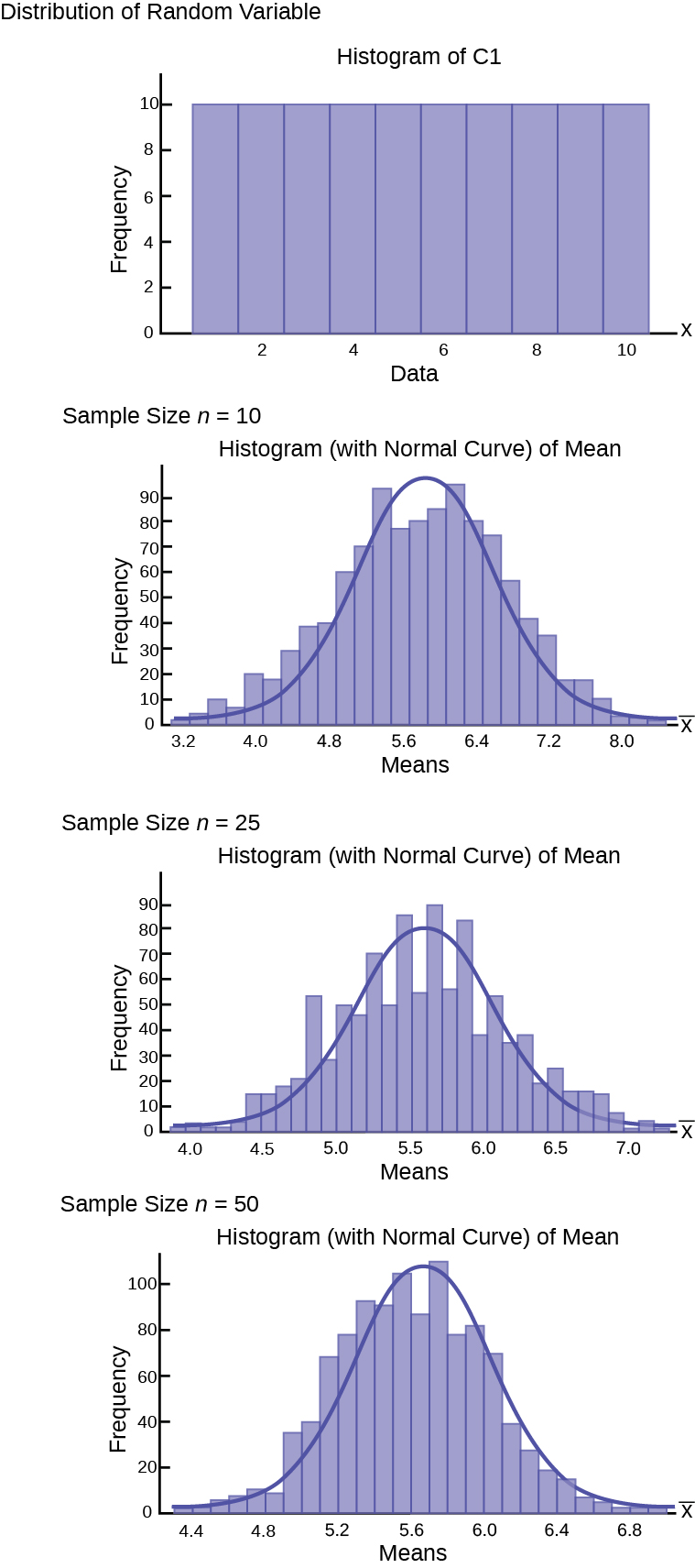
Here are three examples of very different population distributions and the evolution of the sampling distribution to a normal distribution as the sample size increases. The top panel in these cases represents the histogram for the original data. The three panels show the histograms for 1,000 randomly drawn samples for different sample sizes: n=10, n= 25 and n=50. As the sample size increases, and the number of samples taken remains constant, the distribution of the 1,000 sample means becomes closer to the smooth line that represents the normal distribution.

[link] is for a normal distribution of individual observations and we would expect the sampling distribution to converge on the normal quickly. The results show this and show that even at a very small sample size the distribution is close to the normal distribution.

[link] is a uniform distribution which, a bit amazingly, quickly approached the normal distribution even with only a sample of 10.

[link] is a skewed distribution. This last one could be an exponential, geometric, or binomial with a small probability of success creating the skew in the distribution. For skewed distributions our intuition would say that this will take larger sample sizes to move to a normal distribution and indeed that is what we observe from the simulation. Nevertheless, at a sample size of 50, not considered a very large sample, the distribution of sample means has very decidedly gained the shape of the normal distribution.