

| << Chapter < Page | Chapter >> Page > |
Using the following experimental values Engineering Science by E. Hughes and C. Hughes, Longman © 1994, (p. 375) , plot a distance-time graph and determine the equation, relating the distance and time for a moving object.
| Distance [m] | Time [s] |
|---|---|
| 0 | 0 |
| 24 | 5 |
| 48 | 10 |
| 72 | 15 |
| 96 | 20 |
Data can be entered as follows:
distance=[0 24 48 72 96];time=[0 5 10 15 20]; we can now plot the data by typing in
plot(time,distance);title('Distance-Time Graph');xlabel('time');ylabel('distance'); at the MATLAB prompt. The following plot is generated, select Tools>Basic Fitting:
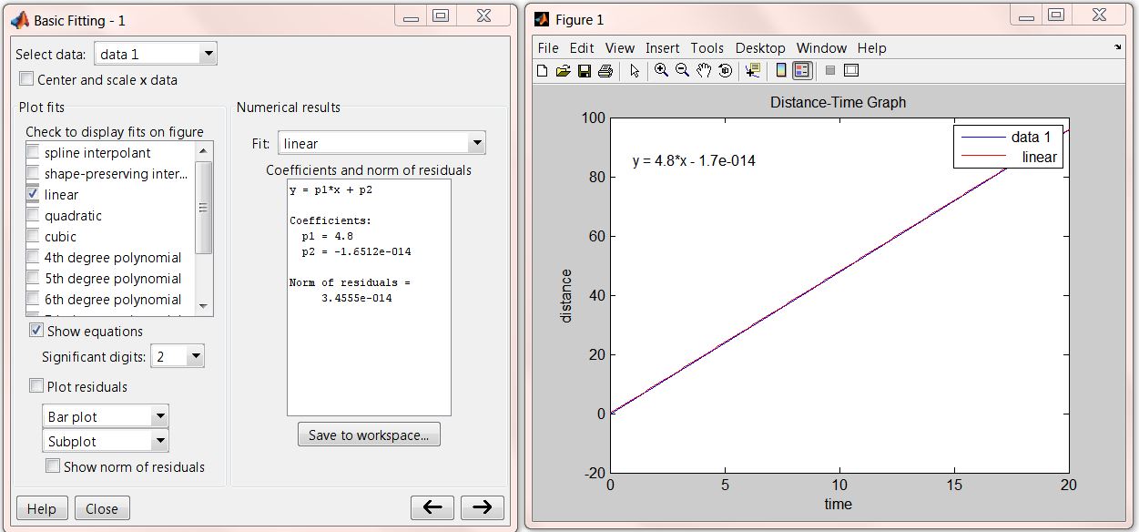
As shown above, the relationship between distance and time is:
or
Using the data set below, determine the relationship between temperature and internal energy.
| Temperature [C] | Internal Energy [kJ/kg] |
|---|---|
| 100 | 2506.7 |
| 150 | 2582.8 |
| 200 | 2658.1 |
| 250 | 2733.7 |
| 300 | 2810.4 |
| 400 | 2967.9 |
| 500 | 3131.6 |
Data can be entered as follows:
temperature = [100, 150, 200, 250, 300, 400, 500];energy = [2506.7, 2582.8, 2658.1, 2733.7, 2810.4, 2967.9, 3131.6]; we can now plot the data by typing in
plot(temperature,energy);title('temperature vs. energy');xlabel('temperature');ylabel('energy'); at the MATLAB prompt. The following plot is generated, select Tools>Basic Fitting:
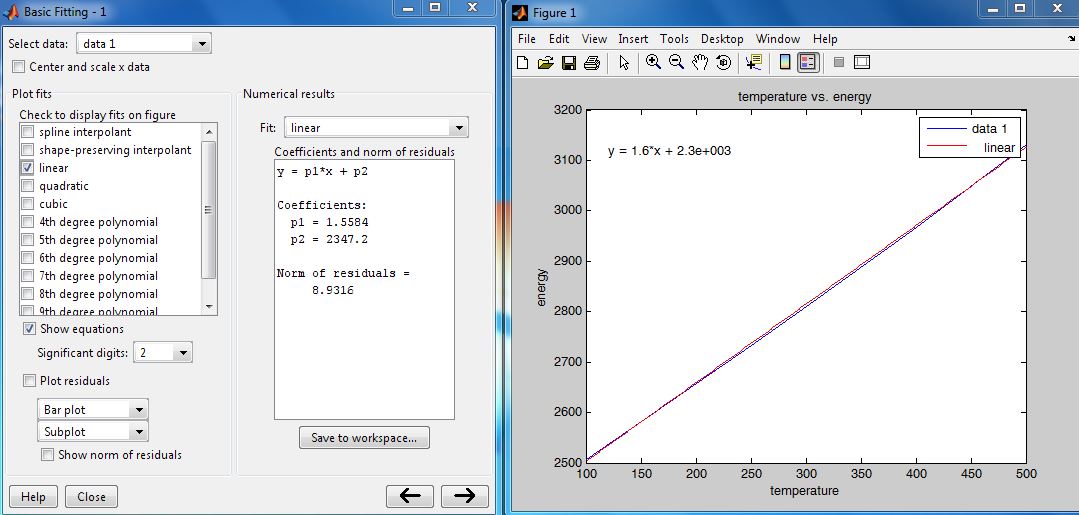
As shown above, the relationship between temperature and internal energy is:
or
Using the following experimental values Engineering Science by E. Hughes and C. Hughes, Longman © 1994, (p. 375) , plot a velocity-time graph and determine the equation, relating the velocity and time for a moving object.
| Velocity [m/s] | Time [s] |
|---|---|
| 12 | 0 |
| 142 | 5 |
| 512 | 10 |
| 1122 | 15 |
| 1972 | 20 |
Data can be entered as follows:
velocity=[12 142 512 1122 1972];time=[0 5 10 15 20]; we can now plot the data by typing in
plot(time,velocity);title('Velocity-Time Graph');xlabel('time');ylabel('velocity'); at the MATLAB prompt. The following plot is generated, select Tools>Basic Fitting, notice that we are choosing the quadratic option this time:
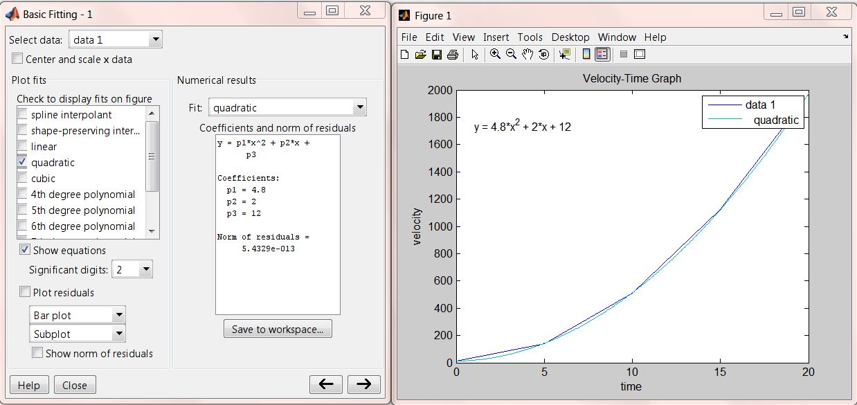
As shown above, the relationship between velocity and time is:
Notification Switch
Would you like to follow the 'A brief introduction to engineering computation with matlab' conversation and receive update notifications?

|
|

|
|

|
|

|
|

|
|

|
|

|
|
|
|
|
|
|
|

|