6.4 Working with taylor series (Page 5/11)

Calculus volume 2 Page 5 / 11

Express $\int cos \sqrt{x} d x$ as an infinite series. Evaluate $\int_{0}^{1} cos \sqrt{x} d x$ to within an error of $0.01 .$

$C + \sum_{n = 1}^{\infty} {(−1)}^{n + 1} \frac{x^{n}}{n (2 n - 2)!}$ The definite integral is approximately $0.514$ to within an error of $0.01 .$

Got questions? Get instant answers now!

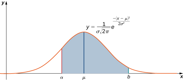
As mentioned above, the integral $\int e^{− x^{2}} d x$ arises often in probability theory. Specifically, it is used when studying data sets that are normally distributed, meaning the data values lie under a bell-shaped curve. For example, if a set of data values is normally distributed with mean $μ$ and standard deviation $σ,$ then the probability that a randomly chosen value lies between $x = a$ and $x = b$ is given by

\frac{1}{σ \sqrt{2 π}} \int_{a}^{b} e^{− {(x - μ)}^{2} / (2 σ^{2})} d x .

(See [link] .)

This graph is the normal distribution. It is a bell-shaped curve with the highest point above mu on the x-axis. Also, there is a shaded area under the curve above the x-axis. The shaded area is bounded by alpha on the left and b on the right. — If data values are normally distributed with mean $μ$ and standard deviation $σ,$ the probability that a randomly selected data value is between $a$ and $b$ is the area under the curve $y = \frac{1}{σ \sqrt{2 π}} e^{− {(x - μ)}^{2} / (2 σ^{2})}$ between $x = a$ and $x = b .$

To simplify this integral, we typically let $z = \frac{x - μ}{σ} .$ This quantity $z$ is known as the $z$ score of a data value. With this simplification, integral [link] becomes

\frac{1}{\sqrt{2 π}} \int_{(a - μ) / σ}^{(b - μ) / σ} e^{− z^{2} / 2} d z .

In [link] , we show how we can use this integral in calculating probabilities.

Using maclaurin series to approximate a probability

Suppose a set of standardized test scores are normally distributed with mean $μ = 100$ and standard deviation $σ = 50 .$ Use [link] and the first six terms in the Maclaurin series for $e^{− x^{2} / 2}$ to approximate the probability that a randomly selected test score is between $x = 100$ and $x = 200 .$ Use the alternating series test to determine how accurate your approximation is.

Since $μ = 100, σ = 50,$ and we are trying to determine the area under the curve from $a = 100$ to $b = 200,$ integral [link] becomes

\frac{1}{\sqrt{2 π}} \int_{0}^{2} e^{− z^{2} / 2} d z .

The Maclaurin series for $e^{− x^{2} / 2}$ is given by

\begin{matrix} e^{− x^{2} / 2} & = \sum_{n = 0}^{\infty} \frac{{(- \frac{x^{2}}{2})}^{n}}{n!} \\ = 1 - \frac{x^{2}}{2^{1} \cdot 1!} + \frac{x^{4}}{2^{2} \cdot 2!} - \frac{x^{6}}{2^{3} \cdot 3!} + ⋯ + {(−1)}^{n} \frac{x^{2 n}}{2^{n} \cdot n!} + ⋯ \\ = \sum_{n = 0}^{\infty} {(−1)}^{n} \frac{x^{2}^{n}}{2^{n} \cdot n!} . \end{matrix}

Therefore,

\begin{matrix} \frac{1}{\sqrt{2 π}} \int e^{− z^{2} / 2} d z & = & \frac{1}{\sqrt{2 π}} \int (1 - \frac{z^{2}}{2^{1} \cdot 1!} + \frac{z^{4}}{2^{2} \cdot 2!} - \frac{z^{6}}{2^{3} \cdot 3!} + ⋯ + {(−1)}^{n} \frac{z^{2 n}}{2^{n} \cdot n!} + ⋯) d z \\ = & \frac{1}{\sqrt{2 π}} (C + z - \frac{z^{3}}{3 \cdot 2^{1} \cdot 1!} + \frac{z^{5}}{5 \cdot 2^{2} \cdot 2!} - \frac{z^{7}}{7 \cdot 2^{3} \cdot 3!} + ⋯ + {(−1)}^{n} \frac{z^{2 n + 1}}{(2 n + 1) 2^{n} \cdot n!} + ⋯) \\ \frac{1}{\sqrt{2 π}} \int_{0}^{2} e^{− z^{2} / 2} d z & = & \frac{1}{\sqrt{2 π}} (2 - \frac{8}{6} + \frac{32}{40} - \frac{128}{336} + \frac{512}{3456} - \frac{2^{11}}{11 \cdot 2^{5} \cdot 5!} + ⋯) . \end{matrix}

Using the first five terms, we estimate that the probability is approximately $0.4922 .$ By the alternating series test, we see that this estimate is accurate to within

\frac{1}{\sqrt{2 π}} \frac{2^{13}}{13 \cdot 2^{6} \cdot 6!} \approx 0.00546 .

Got questions? Get instant answers now!

Use the first five terms of the Maclaurin series for $e^{− x^{2} / 2}$ to estimate the probability that a randomly selected test score is between $100$ and $150 .$ Use the alternating series test to determine the accuracy of this estimate.

The estimate is approximately $0.3414 .$ This estimate is accurate to within $0.0000094 .$

Got questions? Get instant answers now!

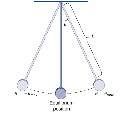
Another application in which a nonelementary integral arises involves the period of a pendulum. The integral is

\int_{0}^{π / 2} \frac{d θ}{\sqrt{1 - k^{2} {sin}^{2} θ}} .

An integral of this form is known as an elliptic integral of the first kind. Elliptic integrals originally arose when trying to calculate the arc length of an ellipse. We now show how to use power series to approximate this integral.

Period of a pendulum

The period of a pendulum is the time it takes for a pendulum to make one complete back-and-forth swing. For a pendulum with length $L$ that makes a maximum angle $θ_{max}$ with the vertical, its period $T$ is given by

T = 4 \sqrt{\frac{L}{g}} \int_{0}^{π / 2} \frac{d θ}{\sqrt{1 - k^{2} {sin}^{2} θ}}

where $g$ is the acceleration due to gravity and $k = sin (\frac{θ_{max}}{2})$ (see [link] ). (We note that this formula for the period arises from a non-linearized model of a pendulum. In some cases, for simplification, a linearized model is used and $sin θ$ is approximated by $θ .)$ Use the binomial series

\frac{1}{\sqrt{1 + x}} = 1 + \sum_{n = 1}^{\infty} \frac{{(−1)}^{n}}{n!} \frac{1 \cdot 3 \cdot 5 ⋯ (2 n - 1)}{2^{n}} x^{n}

to estimate the period of this pendulum. Specifically, approximate the period of the pendulum if

you use only the first term in the binomial series, and
you use the first two terms in the binomial series.

This pendulum has length $L$ and makes a maximum angle $θ_{max}$ with the vertical.

We use the binomial series, replacing $x$ with $− k^{2} {sin}^{2} θ .$ Then we can write the period as

T = 4 \sqrt{\frac{L}{g}} \int_{0}^{π / 2} (1 + \frac{1}{2} k^{2} {sin}^{2} θ + \frac{1 \cdot 3}{2! 2^{2}} k^{4} {sin}^{4} θ + ⋯) d θ .

Using just the first term in the integrand, the first-order estimate is

$T \approx 4 \sqrt{\frac{L}{g}} \int_{0}^{π / 2} d θ = 2 π \sqrt{\frac{L}{g}} .$

If $θ_{max}$ is small, then $k = sin (\frac{θ_{max}}{2})$ is small. We claim that when $k$ is small, this is a good estimate. To justify this claim, consider

$\int_{0}^{π / 2} (1 + \frac{1}{2} k^{2} {sin}^{2} θ + \frac{1 \cdot 3}{2! 2^{2}} k^{4} {sin}^{4} θ + ⋯) d θ .$

Since $| sin x | \leq 1,$ this integral is bounded by

$\int_{0}^{π / 2} (\frac{1}{2} k^{2} + \frac{1.3}{2! 2^{2}} k^{4} + ⋯) d θ < \frac{π}{2} (\frac{1}{2} k^{2} + \frac{1 \cdot 3}{2! 2^{2}} k^{4} + ⋯) .$

Furthermore, it can be shown that each coefficient on the right-hand side is less than $1$ and, therefore, that this expression is bounded by

$\frac{π k^{2}}{2} (1 + k^{2} + k^{4} + ⋯) = \frac{π k^{2}}{2} \cdot \frac{1}{1 - k^{2}},$

which is small for $k$ small.
For larger values of $θ_{max},$ we can approximate $T$ by using more terms in the integrand. By using the first two terms in the integral, we arrive at the estimate

$\begin{matrix} T & \approx 4 \sqrt{\frac{L}{g}} \int_{0}^{π / 2} (1 + \frac{1}{2} k^{2} {sin}^{2} θ) d θ \\ = 2 π \sqrt{\frac{L}{g}} (1 + \frac{k^{2}}{4}) . \end{matrix}$

Got questions? Get instant answers now!

<< Chapter < Page Page > Chapter >>

Practice Key Terms 2

Read also:

Get Jobilize Job Search Mobile App in your pocket Now!

100% Free Mobile Applications
Receive real-time job alerts and never miss the right job again

Source: OpenStax, Calculus volume 2. OpenStax CNX. Feb 05, 2016 Download for free at http://cnx.org/content/col11965/1.2

Google Play and the Google Play logo are trademarks of Google Inc.

Notification Switch

Would you like to follow the 'Calculus volume 2' conversation and receive update notifications?

Ask

©flickr: Iqbal	Liver Cancer By Darlene Paliswat Start Test
	15 Biology 15 Genes and Proteins MCQ By OpenStax Start Quiz
	2 Business Law MCQ 2 By Maureen Miller Start Exam
	Clinical Issues in TB Management By Cath Yu Start Quiz
	11 AP 11 Muscular System MCQ By OpenStax Start Quiz
	12 Biology 12 Mendel's Experiments Heredity MCQ By OpenStax Start Quiz
	4 Pharmacology Essay Excl. Nervous System By Rohini Ajay Start Test
	Business fundamentals By OpenStax Read Online Course
	2 SCEA Java Architect By JavaChamp Team Start Exam
	Economy Foundations By Robert Murphy Start Test