<< Chapter < Page Chapter >> Page >
C P d x + Q d y = C F · T d s ,

this version of Green’s theorem is sometimes referred to as the tangential form of Green’s theorem .

The proof of Green’s theorem is rather technical, and beyond the scope of this text. Here we examine a proof of the theorem in the special case that D is a rectangle. For now, notice that we can quickly confirm that the theorem is true for the special case in which F = P , Q is conservative. In this case,

C P d x + Q d y = 0

because the circulation is zero in conservative vector fields. By [link] , F satisfies the cross-partial condition, so P y = Q x . Therefore,

D ( Q x P y ) d A = D 0 d A = 0 = C P d x + Q d y ,

which confirms Green’s theorem in the case of conservative vector fields.

Proof

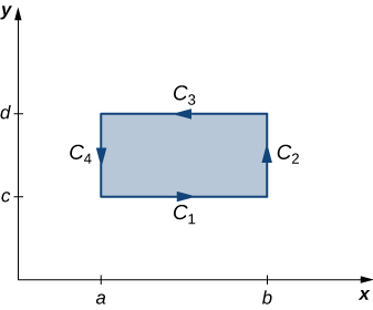
Let’s now prove that the circulation form of Green’s theorem is true when the region D is a rectangle. Let D be the rectangle [ a , b ] × [ c , d ] oriented counterclockwise. Then, the boundary C of D consists of four piecewise smooth pieces C 1 , C 2 , C 3 , and C 4 ( [link] ). We parameterize each side of D as follows:

C 1 : r 1 ( t ) = t , c , a t b C 2 : r 2 ( t ) = b , t , c t d C 3 : r 3 ( t ) = t , d , a t b C 4 : r 4 ( t ) = a , t , c t d .
A diagram in quadrant 1. Rectangle D is oriented counterclockwise. Points a and b are on the x axis, and points c and d are on the y axis with b > a and d > c. The sides of the rectangle are side c1 with endpoints at (a,c) and (b,c), side c2 with endpoints at (b,c) and (b,d), side c3 with endpoints at (b,d) and (a,d), and side c4 with endpoints at (a,d) and (a,c).
Rectangle D is oriented counterclockwise.

Then,

C F d r = C 1 F d r + C 2 F d r + C 3 F d r + C 4 F d r = C 1 F d r + C 2 F d r C 3 F d r C 4 F d r = a b F ( r 1 ( t ) ) r 1 ( t ) d t + c d F ( r 2 ( t ) ) r 2 ( t ) d t a b F ( r 3 ( t ) ) r 3 ( t ) d t c d F ( r 4 ( t ) ) r 4 ( t ) d t = a b P ( t , c ) d t + c d Q ( b , t ) d t a b P ( t , d ) d t c d Q ( a , t ) d t = a b ( P ( t , c ) P ( t , d ) ) d t + c d ( Q ( b , t ) Q ( a , t ) ) d t = a b ( P ( t , d ) P ( t , c ) ) d t + c d ( Q ( b , t ) Q ( a , t ) ) d t .

By the Fundamental Theorem of Calculus,

P ( t , d ) P ( t , c ) = c d y P ( t , y ) d y and Q ( b , t ) Q ( a , t ) = a b x Q ( x , t ) d x .

Therefore,

a b ( P ( t , d ) P ( t , c ) ) d t + c d ( Q ( b , t ) Q ( a , t ) ) d t = a b c d y P ( t , y ) d y d t + c d a b x Q ( x , t ) d x d t .

But,

a b c d y P ( t , y ) d y d t + c d a b x Q ( x , t ) d x d t = a b c d y P ( x , y ) d y d x + c d a b x Q ( x , y ) d x d y = a b c d ( Q x P y ) d y d x = D ( Q x P y ) d A .

Therefore, C F d r = D ( Q x P y ) d A and we have proved Green’s theorem in the case of a rectangle.

To prove Green’s theorem over a general region D , we can decompose D into many tiny rectangles and use the proof that the theorem works over rectangles. The details are technical, however, and beyond the scope of this text.

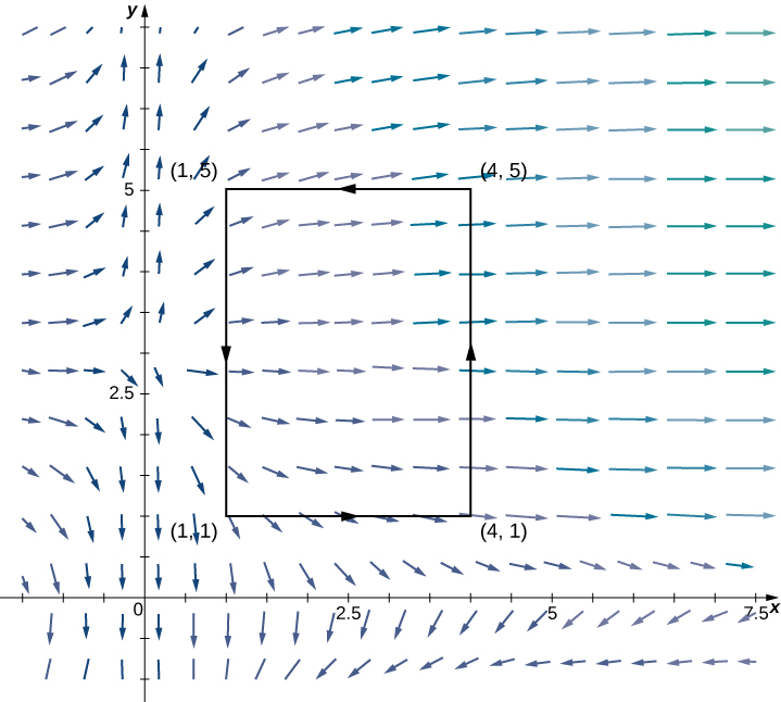
Applying green’s theorem over a rectangle

Calculate the line integral

C x 2 y d x + ( y 3 ) d y ,

where C is a rectangle with vertices ( 1 , 1 ) , ( 4 , 1 ) , ( 4 , 5 ) , and ( 1 , 5 ) oriented counterclockwise.

Let F ( x , y ) = P ( x , y ) , Q ( x , y ) = x 2 y , y 3 . Then, Q x = 0 and P y = x 2 . Therefore, Q x P y = x 2 .

Let D be the rectangular region enclosed by C ( [link] ). By Green’s theorem,

C x 2 y d x + ( y 3 ) d y = D ( Q x P y ) d A = D x 2 d A = 1 5 1 4 x 2 d x d y = 1 5 −21 d y = −84.
A vector field in two dimensions with focus on quadrant 1. The arrows near the origin are short, and the arrows further away from the origin are longer. A rectangle has endpoints at (1,1), (4,1), (4,5), and (1,5). The arrows in quadrant 3 are pointing to the right. At the y axis, they split at y = 3. Arrows above that line curve up at the y axis and shift until they are horizontally pointing to the right in quadrant 1. Arrows below that line and above the x axis curve down at the y axis and shift until they are horizontally pointing to the right. Arrows below the x axis point to the left and down, pointing back to the y axis.
The line integral over the boundary of the rectangle can be transformed into a double integral over the rectangle.
Got questions? Get instant answers now!

Applying green’s theorem to calculate work

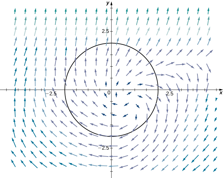
Calculate the work done on a particle by force field

F ( x , y ) = y + sin x , e y x

as the particle traverses circle x 2 + y 2 = 4 exactly once in the counterclockwise direction, starting and ending at point ( 2 , 0 ) .

Let C denote the circle and let D be the disk enclosed by C . The work done on the particle is

W = C ( y + sin x ) d x + ( e y x ) d y .

As with [link] , this integral can be calculated using tools we have learned, but it is easier to use the double integral given by Green’s theorem ( [link] ).

Let F ( x , y ) = P ( x , y ) , Q ( x , y ) = y + sin x , e y x . Then, Q x = −1 and P y = 1 . Therefore, Q x P y = −2 .

By Green’s theorem,

W = C ( y + sin ( x ) ) d x + ( e y x ) d y = D ( Q x P y ) d A = D −2 d A = −2 ( area ( D ) ) = −2 π ( 2 2 ) = −8 π .
A vector field in two dimensions. The arrows further away from the origin are much longer than those near the origin. The arrows curve out from about (.5,.5) in a clockwise spiral pattern.
The line integral over the boundary circle can be transformed into a double integral over the disk enclosed by the circle.
Got questions? Get instant answers now!
Practice Key Terms 2

Get Jobilize Job Search Mobile App in your pocket Now!

Get it on Google Play Download on the App Store Now


Source:  OpenStax, Calculus volume 3. OpenStax CNX. Feb 05, 2016 Download for free at http://legacy.cnx.org/content/col11966/1.2
Google Play and the Google Play logo are trademarks of Google Inc.

Notification Switch

Would you like to follow the 'Calculus volume 3' conversation and receive update notifications?

Ask