<< Chapter < Page Chapter >> Page >
g ( a ) = f ( x ) f ( a ) f ( a ) ( x a ) f ( a ) 2 ! ( x a ) 2 + + f ( n ) ( a ) n ! ( x a ) n R n ( x ) = f ( x ) p n ( x ) R n ( x ) = 0 , g ( x ) = f ( x ) f ( x ) 0 0 = 0.

Therefore, g satisfies Rolle’s theorem, and consequently, there exists c between a and x such that g ( c ) = 0 . We now calculate g . Using the product rule, we note that

d d t [ f ( n ) ( t ) n ! ( x t ) n ] = f ( n ) ( t ) ( n 1 ) ! ( x t ) n 1 + f ( n + 1 ) ( t ) n ! ( x t ) n .

Consequently,

g ( t ) = f ( t ) + [ f ( t ) f ( t ) ( x t ) ] + [ f ( t ) ( x t ) f ( t ) 2 ! ( x t ) 2 ] + + [ f ( n ) ( t ) ( n 1 ) ! ( x t ) n 1 f ( n + 1 ) ( t ) n ! ( x t ) n ] + ( n + 1 ) R n ( x ) ( x t ) n ( x a ) n + 1 .

Notice that there is a telescoping effect. Therefore,

g ( t ) = f ( n + 1 ) ( t ) n ! ( x t ) n + ( n + 1 ) R n ( x ) ( x t ) n ( x a ) n + 1 .

By Rolle’s theorem, we conclude that there exists a number c between a and x such that g ( c ) = 0 . Since

g ( c ) = f ( n + 1 ) ( c ) n ! ( x c ) n + ( n + 1 ) R n ( x ) ( x c ) n ( x a ) n + 1

we conclude that

f ( n + 1 ) ( c ) n ! ( x c ) n + ( n + 1 ) R n ( x ) ( x c ) n ( x a ) n + 1 = 0 .

Adding the first term on the left-hand side to both sides of the equation and dividing both sides of the equation by n + 1 , we conclude that

R n ( x ) = f ( n + 1 ) ( c ) ( n + 1 ) ! ( x a ) n + 1

as desired. From this fact, it follows that if there exists M such that | f ( n + 1 ) ( x ) | M for all x in I , then

| R n ( x ) | M ( n + 1 ) ! | x a | n + 1 .

Not only does Taylor’s theorem allow us to prove that a Taylor series converges to a function, but it also allows us to estimate the accuracy of Taylor polynomials in approximating function values. We begin by looking at linear and quadratic approximations of f ( x ) = x 3 at x = 8 and determine how accurate these approximations are at estimating 11 3 .

Using linear and quadratic approximations to estimate function values

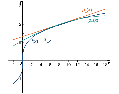
Consider the function f ( x ) = x 3 .

  1. Find the first and second Taylor polynomials for f at x = 8 . Use a graphing utility to compare these polynomials with f near x = 8 .
  2. Use these two polynomials to estimate 11 3 .
  3. Use Taylor’s theorem to bound the error.
  1. For f ( x ) = x 3 , the values of the function and its first two derivatives at x = 8 are as follows:
    f ( x ) = x 3 f ( 8 ) = 2 f ( x ) = 1 3 x 2 / 3 f ( 8 ) = 1 12 f ( x ) = −2 9 x 5 / 3 f ( 8 ) = 1 144 .

    Thus, the first and second Taylor polynomials at x = 8 are given by
    p 1 ( x ) = f ( 8 ) + f ( 8 ) ( x 8 ) = 2 + 1 12 ( x 8 ) p 2 ( x ) = f ( 8 ) + f ( 8 ) ( x 8 ) + f ( 8 ) 2 ! ( x 8 ) 2 = 2 + 1 12 ( x 8 ) 1 288 ( x 8 ) 2 .

    The function and the Taylor polynomials are shown in [link] .
    This graph has four curves. The first is the function f(x)=cube root of x. The second function is psub1(x). The third is psub2(x). The curves are very close around x=8.
    The graphs of f ( x ) = x 3 and the linear and quadratic approximations p 1 ( x ) and p 2 ( x ) .
  2. Using the first Taylor polynomial at x = 8 , we can estimate
    11 3 p 1 ( 11 ) = 2 + 1 12 ( 11 8 ) = 2.25 .

    Using the second Taylor polynomial at x = 8 , we obtain
    11 3 p 2 ( 11 ) = 2 + 1 12 ( 11 8 ) 1 288 ( 11 8 ) 2 = 2.21875 .
  3. By [link] , there exists a c in the interval ( 8 , 11 ) such that the remainder when approximating 11 3 by the first Taylor polynomial satisfies
    R 1 ( 11 ) = f ( c ) 2 ! ( 11 8 ) 2 .

    We do not know the exact value of c , so we find an upper bound on R 1 ( 11 ) by determining the maximum value of f on the interval ( 8 , 11 ) . Since f ( x ) = 2 9 x 5 / 3 , the largest value for | f ( x ) | on that interval occurs at x = 8 . Using the fact that f ( 8 ) = 1 144 , we obtain
    | R 1 ( 11 ) | 1 144 · 2 ! ( 11 8 ) 2 = 0.03125 .

    Similarly, to estimate R 2 ( 11 ) , we use the fact that
    R 2 ( 11 ) = f ( c ) 3 ! ( 11 8 ) 3 .

    Since f ( x ) = 10 27 x 8 / 3 , the maximum value of f on the interval ( 8 , 11 ) is f ( 8 ) 0.0014468 . Therefore, we have
    | R 2 ( 11 ) | 0.0011468 3 ! ( 11 8 ) 3 0.0065104 .
Got questions? Get instant answers now!

Find the first and second Taylor polynomials for f ( x ) = x at x = 4 . Use these polynomials to estimate 6 . Use Taylor’s theorem to bound the error.


p 1 ( x ) = 2 + 1 4 ( x 4 ) ; p 2 ( x ) = 2 + 1 4 ( x 4 ) 1 64 ( x 4 ) 2 ; p 1 ( 6 ) = 2.5 ; p 2 ( 6 ) = 2.4375 ;

| R 1 ( 6 ) | 0.0625 ; | R 2 ( 6 ) | 0.015625

Got questions? Get instant answers now!
Practice Key Terms 5

Get Jobilize Job Search Mobile App in your pocket Now!

Get it on Google Play Download on the App Store Now


Source:  OpenStax, Calculus volume 2. OpenStax CNX. Feb 05, 2016 Download for free at http://cnx.org/content/col11965/1.2
Google Play and the Google Play logo are trademarks of Google Inc.

Notification Switch

Would you like to follow the 'Calculus volume 2' conversation and receive update notifications?

Ask