<< Chapter < Page Chapter >> Page >

Find the value of C ( x = y ) d s , where C is the curve parameterized by x = t , y = t , 0 t 1 .

2

Got questions? Get instant answers now!

Note that in a scalar line integral, the integration is done with respect to arc length s , which can make a scalar line integral difficult to calculate. To make the calculations easier, we can translate C f d s to an integral with a variable of integration that is t .

Let r ( t ) = x ( t ) , y ( t ) , z ( t ) for a t b be a parameterization of C . Since we are assuming that C is smooth, r ( t ) = x ( t ) , y ( t ) , z ( t ) is continuous for all t in [ a , b ] . In particular, x ( t ) , y ( t ) , and z ( t ) exist for all t in [ a , b ] . According to the arc length formula, we have
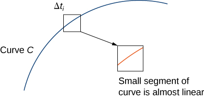
length ( C i ) = Δ s i = t i 1 t i r ( t ) d t .

If width Δ t i = t i t i 1 is small, then function t i 1 t i r ( t ) d t r ( t i * ) Δ t i , r ( t ) is almost constant over the interval [ t i 1 , t i ] . Therefore,

t i 1 t i r ( t ) d t r ( t i * ) Δ t i ,

and we have

i = 1 n f ( r ( t i * ) ) Δ s i = i = 1 n f ( r ( t i * ) ) r ( t i * ) Δ t i .

See [link] .

A segment of an increasing concave down curve labeled C. A small segment of the curved is boxed and labeled as delta t_i. In the zoomed-in insert, this boxed segment of the curve is almost linear.
If we zoom in on the curve enough by making Δ t i very small, then the corresponding piece of the curve is approximately linear.

Note that

lim n i = 1 n f ( r ( t i * ) ) r ( t i * ) Δ t i = a b f ( r ( t ) ) r ( t ) d t .

In other words, as the widths of intervals [ t i 1 , t i ] shrink to zero, the sum i = 1 n f ( r ( t i * ) ) r ( t i * ) Δ t i converges to the integral a b f ( r ( t ) ) r ( t ) d t . Therefore, we have the following theorem.

Evaluating a scalar line integral

Let f be a continuous function with a domain that includes the smooth curve C with parameterization r ( t ) , a t b . Then

C f d s = a b f ( r ( t ) ) r ( t ) d t .

Although we have labeled [link] as an equation, it is more accurately considered an approximation because we can show that the left-hand side of [link] approaches the right-hand side as n . In other words, letting the widths of the pieces shrink to zero makes the right-hand sum arbitrarily close to the left-hand sum. Since

r ( t ) = ( x ( t ) ) 2 + ( y ( t ) ) 2 + ( z ( t ) ) 2 ,

we obtain the following theorem, which we use to compute scalar line integrals.

Scalar line integral calculation

Let f be a continuous function with a domain that includes the smooth curve C with parameterization r ( t ) = x ( t ) , y ( t ) , z ( t ) , a t b . Then

C f ( x , y , z ) d s = a b f ( r ( t ) ) = ( x ( t ) ) 2 + ( y ( t ) ) 2 + ( z ( t ) ) 2 d t .

Similarly,

C f ( x , y ) d s = a b f ( r ( t ) ) = ( x ( t ) ) 2 + ( y ( t ) ) 2 d t

if C is a planar curve and f is a function of two variables.

Note that a consequence of this theorem is the equation d s = r ( t ) d t . In other words, the change in arc length can be viewed as a change in the t domain, scaled by the magnitude of vector r ( t ) .

Evaluating a line integral

Find the value of integral C ( x 2 + y 2 + z ) d s , where C is part of the helix parameterized by r ( t ) = cos t , sin t , t , 0 t 2 π .

To compute a scalar line integral, we start by converting the variable of integration from arc length s to t . Then, we can use [link] to compute the integral with respect to t . Note that f ( r ( t ) ) = cos 2 t + sin 2 t + t = 1 + t and

( x ( t ) ) 2 + ( y ( t ) ) 2 + ( z ( t ) ) 2 = ( sin ( t ) ) 2 + cos 2 ( t ) + 1 = 2 .

Therefore,

C ( x 2 + y 2 + z ) d s = 0 2 π ( 1 + t ) 2 d t .

Notice that [link] translated the original difficult line integral into a manageable single-variable integral. Since

0 2 π ( 1 + t ) 2 d t = [ 2 t + 2 t 2 2 ] 0 2 π = 2 2 π + 2 2 π 2 ,

we have

C ( x 2 + y 2 + z ) d s = 2 2 π + 2 2 π 2 .
Got questions? Get instant answers now!

Evaluate C ( x 2 + y 2 + z ) d s , where C is the curve with parameterization r ( t ) = sin ( 3 t ) , cos ( 3 t ) , 0 t π 4 .

1 3 + 2 6 + 3 π 4

Got questions? Get instant answers now!
Practice Key Terms 8

Get Jobilize Job Search Mobile App in your pocket Now!

Get it on Google Play Download on the App Store Now


Source:  OpenStax, Calculus volume 3. OpenStax CNX. Feb 05, 2016 Download for free at http://legacy.cnx.org/content/col11966/1.2
Google Play and the Google Play logo are trademarks of Google Inc.

Notification Switch

Would you like to follow the 'Calculus volume 3' conversation and receive update notifications?

Ask