

| << Chapter < Page | Chapter >> Page > |
Suppose X is a random variable with a distribution that may be known or unknown (it can be any distribution). Using a subscript that matches the random variable, suppose:
If you draw random samples of size n , then as n increases, the random variable which consists of sample means, tends to be normally distributed and
~ N .
The central limit theorem for sample means says that if you keep drawing larger and larger samples (such as rolling one, two, five, and finally, ten dice) and calculating their means, the sample means form their own normal distribution (the sampling distribution). The normal distribution has the same mean as the original distribution and a variance that equals the original variance divided by, the sample size. The variable n is the number of values that are averaged together, not the number of times the experiment is done.
To put it more formally, if you draw random samples of size n , the distribution of the random variable , which consists of sample means, is called the sampling distribution of the mean . The sampling distribution of the mean approaches a normal distribution as n , the sample size , increases.
The random variable has a different z -score associated with it from that of the random variable X . The mean is the value of in one sample.
μ X is the average of both X and .
= standard deviation of and is called the standard error of the mean.
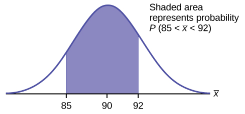
An unknown distribution has a mean of 90 and a standard deviation of 15. Samples of size n = 25 are drawn randomly from the population.
a. Find the probability that the
sample mean is between 85 and 92.
a. Let X = one value from the original unknown population. The probability question asks you to find a probability for the sample mean .
Let = the mean of a sample of size 25. Since μ X = 90, σ X = 15, and n = 25,
~ N .
Find P (85< <92). Draw a graph.
P (85< <92) = 0.6997
The probability that the sample mean is between 85 and 92 is 0.6997.
b. Find the value that is two standard deviations above the expected value, 90, of the sample mean.
b. To find the value that is two standard deviations above the expected value 90, use the formula:
value = μ x + (#ofTSDEVs)
value = 90 + 2 = 96
The value that is two standard deviations above the expected value is 96.
The standard error of the mean is = = 3. Recall that the standard error of the mean is a description of how far (on average) that the sample mean will be from the population mean in repeated simple random samples of size n .
An unknown distribution has a mean of 45 and a standard deviation of eight. Samples of size n = 30 are drawn randomly from the population. Find the probability that the sample mean is between 42 and 50.
P (42< <50) = = 0.9797
The length of time, in hours, it takes an "over 40" group of people to play one soccer match is normally distributed with a mean of two hours and a standard deviation of 0.5 hours . A sample of size n = 50 is drawn randomly from the population. Find the probability that the sample mean is between 1.8 hours and 2.3 hours.
Let X = the time, in hours, it takes to play one soccer match.
The probability question asks you to find a probability for the sample mean time, in hours , it takes to play one soccer match.
Let = the mean time, in hours, it takes to play one soccer match.
If μ X = _________, σ X = __________, and n = ___________, then X ~ N (______, ______) by the central limit theorem for means .
μ X = 2, σ X = 0.5, n = 50, and X ~ N
Find P (1.8< <2.3). Draw a graph.
P (1.8< <2.3) = 0.9977
The probability that the mean time is between 1.8 hours and 2.3 hours is 0.9977.
Notification Switch
Would you like to follow the 'Statistics i - math1020 - red river college - version 2015 revision a - draft 2015-10-24' conversation and receive update notifications?

|
|

|
|

|
|

|
|

|
|

|
|

|
|

|
|

|
|

|