

| << Chapter < Page | Chapter >> Page > |
The word matrix dates at least to the thirteenth century, when it was used to describe the rectangular copper tray, or matrix, that held individual leaden letters that were packed into the matrix to form a page of composed text. Each letter in the matrix, call it , occupied a unique position in the matrix. In modern day mathematical parlance, a matrix is a collection of numbers arranged in a two-dimensional array (a rectangle). We indicate a matrix with a boldfaced capital letter and the constituent elements with double subscripts for the row and column:
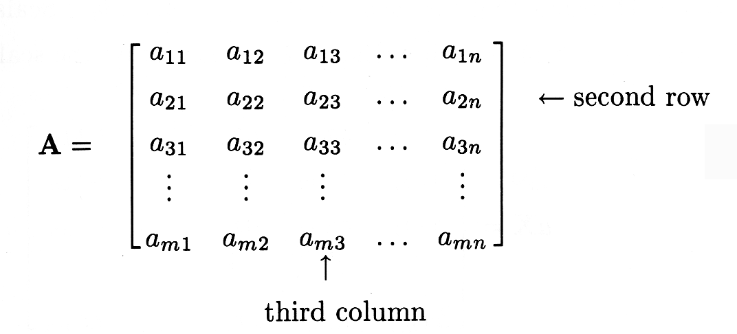
In this equation is an matrix, meaning that has horizontal rows and vertical columns. As an extension of the previously used notation, we write to show that is a matrix of size with . The scalar element is located in the matrix at the row and the column. For example, is located in the second row and the third column as illustrated in [link] .
The main diagonal of any matrix consists of the elements . (The two subscripts are equal.) The main diagonal runs southeast from the top leftcorner of the matrix, but it does not end in the lower right corner unless the matrix is square .
The
transpose of a matrix
is another matrix
whose
element in row
and column
is
for
and
.
We write
to indicate that
is the transpose of
. In MATLAB,
transpose is denoted by. A more intuitive way of describing the transpose
operation is to say that it flips the matrix about its main diagonal so thatrows become columns and columns become rows.
A'
Matrix Addition and Scalar Multiplication. Two matrices of the same size (in both dimensions) may be added or subtracted in the same way as vectors, by adding or subtracting the corresponding elements. The equation means that for each i and . Scalar multiplication of a matrix multiplies each element of the matrix by the scalar:
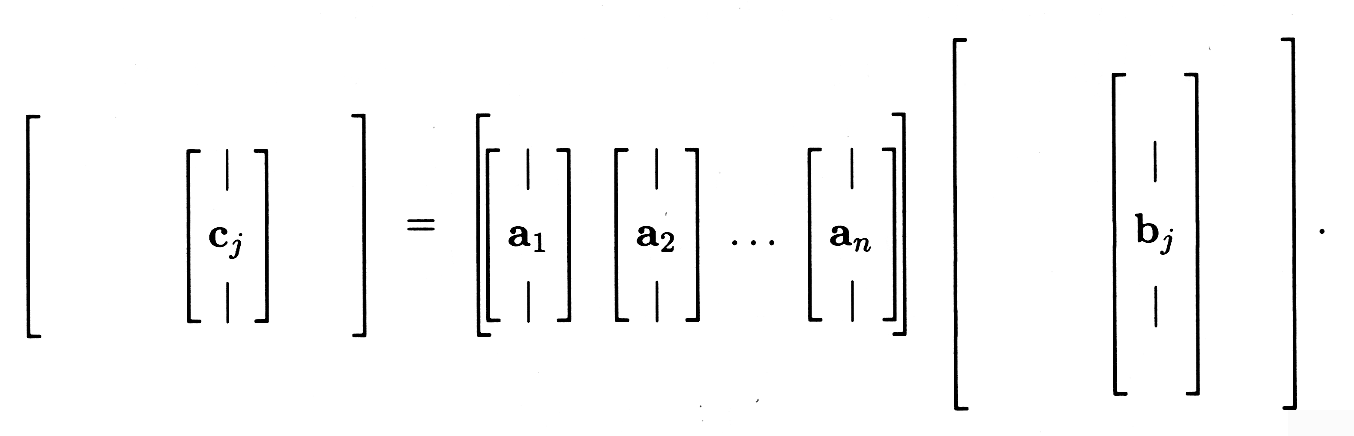
Matrix Multiplication. A vector can be considered a matrix with only one column. Thus we intentionally blur the distinction between and R n . Also a matrix can be viewed as a collection of vectors, each column of the matrix being a vector:
In the transpose operation, columns become rows and vice versa. The transpose of an matrix, a column vector , is a 1 matrix, a row vector :
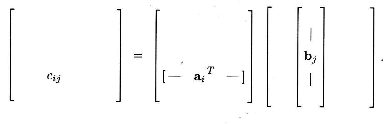
Now we can define matrix-matrix multiplication in terms of inner products of vectors. Let's begin with matrices and . To find the product AB, first divide each matrix into column vectors and row vectors as follows:
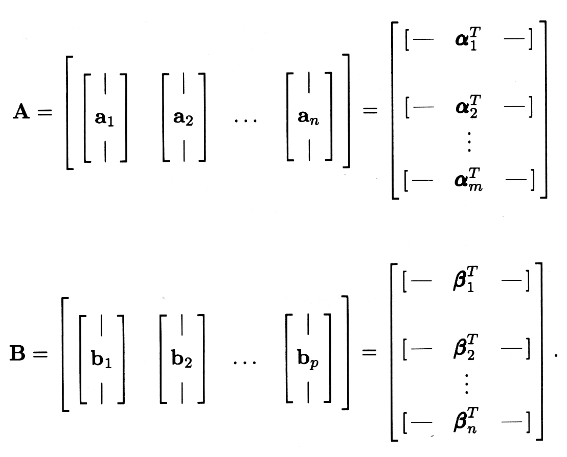
Thus is the column of A and is the row of A. For matrix multiplication to be defined, the width of the first matrix must match thelength of the second one so that all rows and columns have the same number of elements . The matrix product, AB, is an matrix defined by its elements as . In words, each element of the product matrix, , is the inner product of the row of the first matrix and the column of the second matrix.
For n-vectors and , the matrix product takes on a special significance. The product is, of course, a matrix (a scalar). The special significance is that is the inner product of and :
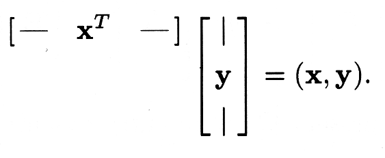
Thus the notation
is often used in place of
. Recall from
Demo 1 from "Linear Algebra: Other Norms" that MATLAB usesto denote inner product.
x'*y
Another special case of matrix multiplication is the outer product . Like the inner product, it involves two vectors, but this time the result is a matrix:
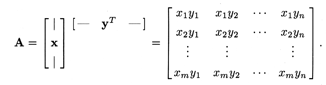
In the outer product, the inner products that define its elements are between one-dimensional row vectors of and one-dimensional column vectors of , meaning the element of is .
There are several other equivalent ways to define matrix multiplication, and a careful study of the following discussion should improve your understanding of matrix multiplication. Consider A , and so that . In pictures, we have
In our definition, we represent on an entry-by-entry basis as
In pictures,
You will prove in Exercise 3 that we can also represent on a column basis:
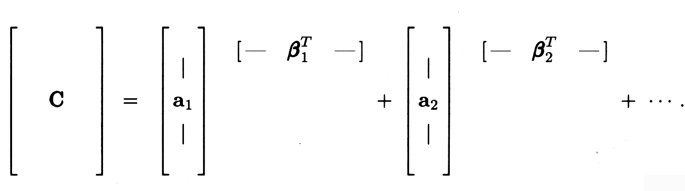
Finally, can be represented as a sum of matrices, each matrix being an outer product:
A numerical example should help clarify these three methods.
Let
Using the first method of matrix multiplication, on an entry-by-entry basis, we have
or
or
On a column basis,
Collecting terms together, we have
On a matrix-by-matrix basis,
as we had in each of the other cases. Thus we see that the methods are equivalent-simply different ways of organizing the same computation!
We know from the chapter on complex numbers that a complex number may be rotated by angle in the complex plane by forming the product
When written out, the real and imaginary parts of are
If the real and imaginary parts of and are organized into vectors and as in the chapter on complex numbers , then rotation may be carried out with the matrix-vector multiply
We call the matrix a rotation matrix .
Notification Switch
Would you like to follow the 'A first course in electrical and computer engineering' conversation and receive update notifications?

|
|

|
|

|
|

|
|

|
|

|
|

|
|

|
|

|
|

|