5.4 Continuous wavelet transform

The STFT provided a means of (joint) time-frequency analysis with the property that spectral/temporal widths (or resolutions)were the same for all basis elements. Let's now take a closer look at the implications of uniform resolution.

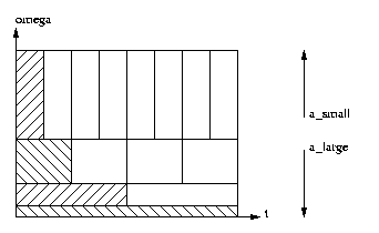
Consider two signals composed of sinusoids with frequency 1 Hz and 1.001 Hz, respectively. It may be difficult to distinguishbetween these two signals in the presence of background noise unless many cycles are observed, implying the need for amany-second observation. Now consider two signals with pure frequencies of 1000 Hz and 1001 Hz-again, a 0.1%difference. Here it should be possible to distinguish the two signals in an interval of much less than one second. In otherwords, good frequency resolution requires longer observation times as frequency decreases. Thus, it might be more convenientto construct a basis whose elements have larger temporal width at low frequencies.

The previous example motivates a multi-resolution time-frequency tiling of the form ( [link] ):

The Continuous Wavelet Transform (CWT) accomplishes the above multi-resolution tiling by time-scaling and time-shifting aprototype function $\psi (t)$ , often called the mother wavelet . The $a$ -scaled and $\tau$ -shifted basis elements is given by $${\psi }_{a,\tau }(t)=\frac{1}{\sqrt{\left|a\right|}}\psi (\frac{t-\tau }{a})$$ where $$(a\land \tau )\in \mathbb{R}$$ $$\int_{()} \,d t$$∞ ∞ ψ t 0 $$C_{\psi }=\int_{()} \,d \Omega$$∞ ∞ ψ Ω 2 Ω ∞ The conditions above imply that $\psi (t)$ is bandpass and sufficiently smooth. Assuming that $(\psi (t))=1$ , the definition above ensures that $({\psi }_{a,\tau }(t))=1$ for all $a$ and $\tau$ . The CWT is then defined by the transform pair $$X_{\mathrm{CWT}}(a, \tau )=\int_{()} \,d t$$∞ ∞ x t ψ a , τ t $$x(t)=\frac{1}{C_{\psi }}\int_{()} \,d a$$∞ ∞ τ ∞ ∞ X CWT a τ ψ a , τ t a 2 In basis terms, the CWT says that a waveform can be decomposed into a collection of shifted and stretched versions of themother wavelet $\psi (t)$ . As such, it is usually said that wavelets perform a "time-scale" analysis rather than a time-frequency analysis.

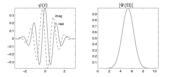
The Morlet wavelet is a classic example of the CWT. It employs a windowed complex exponential as the motherwavelet: $$\psi (t)=\frac{1}{\sqrt{2\pi }}e^{-(i{\Omega }_{0}t)}e^{-\left(\frac{t^2}{2}\right)}$$ $$\Psi (\Omega )=e^{-\left(\frac{(\Omega -{\Omega }_0)^2}{2}\right)}$$ where it is typical to select ${\Omega }_0=\pi \sqrt{\frac{2}{\lg 2}}$ . (See illustration .) While this wavelet does not exactly satisfy the conditions established earlier, since $\Psi (0)\approx 7E-7\neq 0$ , it can be corrected, though in practice the correction is negligible and usually ignored.

While the CWT discussed above is an interesting theoretical and pedagogical tool, the discrete wavelet transform (DWT) is muchmore practical. Before shifting our focus to the DWT, we take a step back and review some of the basic concepts from the branchof mathematics known as Hilbert Space theory ( Vector Space , Normed Vector Space , Inner Product Space , Hilbert Space , Projection Theorem ). These concepts will be essential in our development of the DWT.