5.4 Background on artificial neural network

Motivation:

As the Blind Source Separation algorithm randomly assigns the two independent components into two output vectors, we need the artificial neural network to determine which of the two signals, if any, contains human speech.

Background on Our Chosen Neural Network Model:

Our Neural Networks Model:

A simplified schematics of our neural network looks like the following:

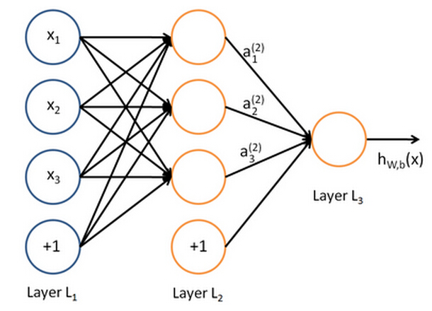
Our artificial neural network consists of one input layer (Layer L1), one hidden layer (Layer L2), and one output layer (Layer L3). The circles labeled “+1” are called the bias units, and corresponds to the intercept term.

Our neural network has parameters ( W , b ) = ( W ⁽¹⁾ , b ⁽¹⁾ , W ⁽²⁾ , b ⁽²⁾ ), where we write W ^(l) _ij to denote the weight associated with the connection between unit j in layer l, and unit i in layer l+1. Also, b ^(l) _i is the bias associated with unit i in layer l+1. We also use s _l to denote the number of nodes in layer l (not counting the bias unit).

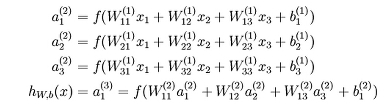
We will write a ^(l) _i to denote the activation of unit i in layer l. For l=1, we also use a ⁽¹⁾ _i =x _i to denote the i-th input. Given a fixed setting of the parameters W,b, our neural network defines a hypothesis h _W,b (x) that outputs a real number. Specifically, the computation that this neural network represents is given by:

Let z ^(l) _i denote the total weighted sum of inputs to unit i in layer l, including the bias unit. For instance, , so that .

If we extend the activation function f(.) to apply to vectors in an element-wise fashion, we can write the above equations more compactly as:

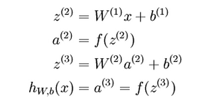
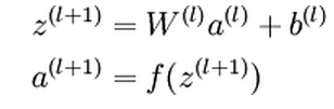
The above equations represents the forward propagation step. More generally, as we use a ⁽¹⁾ =x to denote the values from the input layer, then given layer l’s activations a ^(l) , we can compute layer l+1’s activations a ^(l+1) as:

Backpropagation Algorithm:

Suppose we have a fixed training set of m training examples, the overall cost function is:

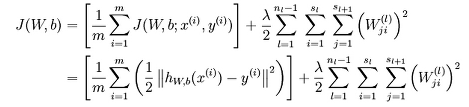
The first term in the cost function is an average sum-of-squares error term. The second term is the regularization term which is used to prevent overfitting. The weight decay parameter λ controls the relative importance of the cost term and the regularization term.

Our goal is to minimize the cost function J(W,b) as a function of W and b. To begin training our neural network, we will initialize each weight W ^(l) _ij and each b ^(l) _i to a small value near zero. It is important to initialize the parameters randomly for the purpose of symmetry breaking.

In order to perform gradient descent to minimize the cost function, we need to compute the derivatives of the cost function with respect to W ^(l) _ij and b ^(l) _i respectively:

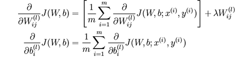
The intuition behind the backpropagation algorithm is as follows. Given a training example (x,y), we will first run a “forward propagation” to compute all the activations, including the output value of the hypothesis h _W,b (x). Then for each node i in layer l, we compute an error term δ ^(l) _i that measures how much that node was responsible for any errors in the output. For an output node, we can directly measure the difference between the network’s hypothesis and the true value, and use that to define the error term for the output layer.

Here is the implementation of the backpropagation algorithm in MatLab:

1. Perform a feedforward propagation, computing the activations for hidden layer L2 and output layer L3.
2. For the output layer (layer n _l ), set

1. For the hidden layer, set

1. Compute the desired partial derivative of the cost function with respect to W and b

Implementation note: in step 2 and 3 above, we need to compute f’(z ^(l) _i ) for each value of i. as our f(z) is the sigmoid function and we already have a ^(l) _i computed during the feedforward propagation process. Thus using the expression for f’(z), we can compute this as .

Below is the pseudo code of the gradient descent algorithm:

Note: ΔW ^(l) is a matrix of the same dimension as W ^(l) and Δb ^(l) is a vector of the same dimension as b ^(l) . one iteration of the gradient descent as follows:

1. Set ΔW ^(l) := 0, Δb ^(l) := 0 for all l.
2. For i from 1 to m,

1. Use backpropagation to compute

1. Set
2. Set

1. Update the parameters:

We can now repeat the gradient descent steps to reduce our cost function J(W,b).