5.3 Blind source separation  (Page 2/2)

The following sections will explain the three filters in detail.

• B(ω) , the separation filter.
• Bm+ , the normalization filter used to solve the scaling problem that arises after applying independent component analysis.
• P(ω) , the permutation filter used to solve the frequency distortion problem that arises after applying independent component analysis.

Separation filter

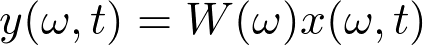
The separation filter, shown in the previous section can be broken down into the following components.

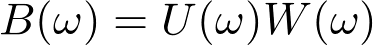
W(ω) is the preprocessing filter used to reduce reflections and ambient noise by using the subspace method. U(ω) is the filter obtained by applying independent component analysis after preprocessing.

I. subspace method

The spatial correlation, or autocorrelation, matrix at frequency ω is defined below.

Given that there are M inputs and M sources, the resulting matrix will be M × M . This matrix can be rewritten in the following way.

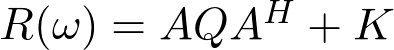
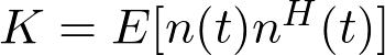
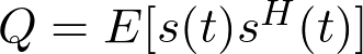
In other words, K is the correlation matrix of n(t) and Q is the cross-spectrum matrix of the sources. However, since the source signals, s(t) , are unknown at this point, this equation cannot be directly solved. Instead, we can represent the generalized eigenvalue decomposition of the spatial correlation matrix in the following manner.

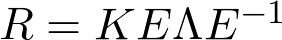
E refers is the eigenvector matrix, E = [e1,e2, …,eM] , and Λ = diag(λ1,λ2,…,λM) refers to the eigenvalues of R . Since K , the noise correlation matrix, cannot be directly observed apart from the source signals, we will assume that K = I , which will evenly distribute the reflections and ambient noise induced by the environment among the estimated sources. As such, the eigenvalue decomposition of R can be rewritten as the following.

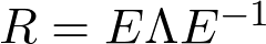
The final preprocessing filter uses the eigevector and eigenvalue matrices resulting from the standard eigenvalue decomposition of the spatial correlation matrix and is shown below.

Ii. independent component analysis

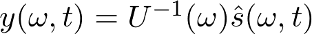
By applying the preprocessing filter obtained from the subspace method, our observed signals are now of the following form.

To estimate the source signals from the preprocessed input signals, we can use independent component analysis to solve the linear system displayed below, for the filter U(ω) .

Now that the separation filter at each frequency has been found, the problems that arise from the separation process must be addressed.

Scaling

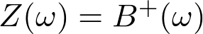
The scaling problem that results from applying independent component analysis can be resolved using the filter shown below.

Bm,n+(ω) refers to the (m,n) th entry in B+(ω) , which is the pseudo-inverse of B(ω) (regular inverse also works here since we assume that the number of separated sources and the number of inputs are both M , so that the resulting separation matrix is square). Additionally, m refers to an arbitrary row or microphone in B+(ω) . By applying this matrix, each signal, i , is amplified by the component of signal i observed at microphone or input m . Essentially, this filter amplifies the frequency components of the separated source signals so that the waveforms of the resulting sources will be distinguishable and audible.

Permutation

A second critical problem that arises after applying independent component analysis is that the order in which the source signals are returned is unknown. Since independent component analysis is applied at each frequency, we must find the permutation of components that has the highest chance of being the correct permutation to reconstruct the source signals and minimize the amount of frequency distortion caused by independent component analysis.

We define the permutation matrix, P , as the following.

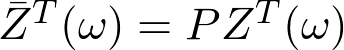
The matrix, P , exchanges the column vectors of Z(ω) to get different permutations. We define the cosine of θn between the two vectors zn(ω) and zn(ω0) , where ω0 is the reference frequency is as follows.

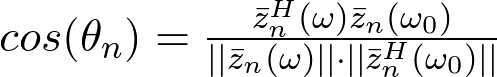
The permutation is, then, determined by the following.

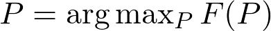
The cost function, F(P) , used above, is defined as follows.

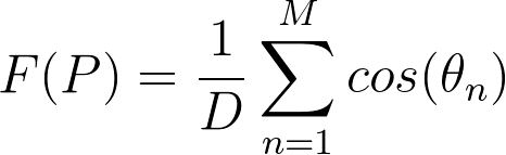
This compares the inverse vector filter at each frequency with a filter at a reference frequency, ω0 . However, if we use the same reference frequency to find the permutation at every other frequency, then the problem arises if the filter at the reference frequency has the incorrect permutation. In order to minimize this error, a new reference frequency is chosen after the permutations of filters at K frequencies are found. As such, the frequency range of a reference frequency, ω0 , is as follows.