

| << Chapter < Page | Chapter >> Page > |
Consider the region in the first quadrant between the functions and ( [link] ). Describe the region first as Type I and then as Type II.
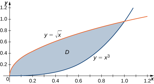
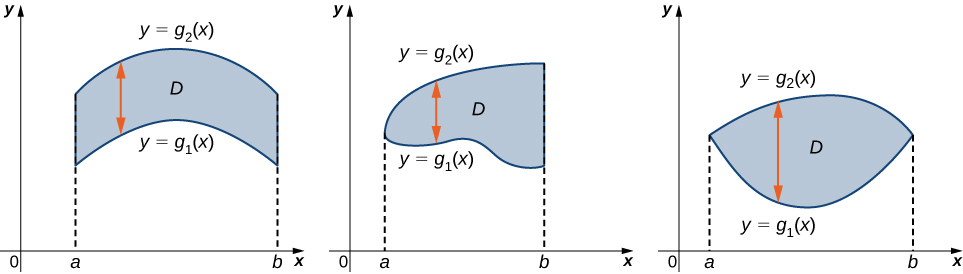
When describing a region as Type I, we need to identify the function that lies above the region and the function that lies below the region. Here, region is bounded above by and below by in the interval for Hence, as Type I, is described as the set
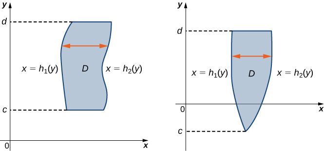
However, when describing a region as Type II, we need to identify the function that lies on the left of the region and the function that lies on the right of the region. Here, the region is bounded on the left by and on the right by in the interval for y in Hence, as Type II, is described as the set
Consider the region in the first quadrant between the functions and Describe the region first as Type I and then as Type II.
Type I and Type II are expressed as and respectively.
To develop the concept and tools for evaluation of a double integral over a general, nonrectangular region, we need to first understand the region and be able to express it as Type I or Type II or a combination of both. Without understanding the regions, we will not be able to decide the limits of integrations in double integrals. As a first step, let us look at the following theorem.
Suppose is the extension to the rectangle of the function defined on the regions and as shown in [link] inside Then is integrable and we define the double integral of over by
The right-hand side of this equation is what we have seen before, so this theorem is reasonable because is a rectangle and has been discussed in the preceding section. Also, the equality works because the values of are for any point that lies outside and hence these points do not add anything to the integral. However, it is important that the rectangle contains the region
As a matter of fact, if the region is bounded by smooth curves on a plane and we are able to describe it as Type I or Type II or a mix of both, then we can use the following theorem and not have to find a rectangle containing the region.
For a function that is continuous on a region of Type I, we have
Similarly, for a function that is continuous on a region of Type II, we have
The integral in each of these expressions is an iterated integral, similar to those we have seen before. Notice that, in the inner integral in the first expression, we integrate with being held constant and the limits of integration being In the inner integral in the second expression, we integrate with being held constant and the limits of integration are
Notification Switch
Would you like to follow the 'Calculus volume 3' conversation and receive update notifications?

|
|

|
|

|
|

|
|

|
|

|
|

|
|

|
|

|
|

|